Bringing Historical Process Data to Life: Unlocking AI’s Goldmine with Neural Networks for Smarter Manufacturing

In every factory, industrial operation, and chemical plant, vast amounts of process data are continuously recorded. Yet most of it remains unused, buried in digital archives. What if we could bring this hidden goldmine to life and transform it into a powerful tool for process optimization, cost reduction, and predictive decision-making? AI and machine learning (ML) are revolutionizing industries by turning raw data into actionable insights. From predicting product quality in real-time to optimizing chemical reactions, AI-driven process modeling is not just the future. It is ready to be implemented today.

In this article, I will explore how historical process data can be extracted, neural networks can be trained, and AI models can be deployed to provide instant and accurate predictions. These technologies will help industries operate smarter, faster, and more efficiently than ever before.

How many years of industrial process data are sitting idle on your company’s servers? It’s time to unleash it—because, with AI, it’s a goldmine.

I personally know of billion-dollar companies that have decades of process data collecting dust. Manufacturing firms have been diligently logging process data through automated DCS (Distributed Control Systems) and PLC (Programmable Logic Controller) systems at millisecond intervals—or even smaller—since the 1980s. With advancements in chip technology, data collection has only become more efficient and cost-effective. Leading automation companies such as Siemens (Simatic PCS 7), Yokogawa (Centum VP), ABB (800xA), Honeywell (Experion), Rockwell Automation (PlantPAx), Schneider Electric (Foxboro), and Emerson (Delta V) have been at the forefront of industrial data and process automation. As a result, massive repositories of historical process data exist within organizations—untapped and underutilized.

Every manufacturing process involves inputs (raw materials and energy) and outputs (products). During processing, variables such as temperature, pressure, motor speeds, energy consumption, byproducts, and chemical properties are continuously logged. Final product metrics—such as yield and purity—are checked for quality control, generating additional data. Depending on the complexity of the process, these parameters can range from just a handful to hundreds or even thousands.

A simple analogy: consider the manufacturing of canned soup. Process variables might include ingredient weights, chunk size distribution, flavoring amounts, cooking temperature and pressure profiles, stirring speed, moisture loss, and can-filling rates. The outputs could be both numerical (batch weight, yield, calories per serving) and categorical (taste quality, consistency ratings). This pattern repeats across industries—whether in chemical plants, refineries, semiconductor manufacturing, pharmaceuticals, food processing, polymers, cosmetics, power generation, or electronics—every operation has a wealth of process data waiting to be explored.

For companies, revenue is driven by product sales. Those that consistently produce high-quality products thrive in the marketplace. Profitability improves when sales increase and when cost of goods sold (COGS) and operational inefficiencies are reduced. Process data can be leveraged to minimize product rejects, optimize yield, and enhance quality—directly impacting the bottom line.

How can AI help?

The answer is simple: AI can process vast amounts of historical data and predict product quality and performance based on input parameters—instantly and with remarkable accuracy.

A Real-Life Manufacturing Scenario

Imagine you’re the VP of Manufacturing at a pharmaceutical company that produces a critical cancer drug—a major revenue driver. You’ve been producing this drug for seven years, ensuring a steady supply to patients worldwide.

Today, a new batch has just finished production. It will take a week for quality testing before final approval. However, a power disruption occurred during the run, requiring process adjustments and minor parts replacements. The process was completed as planned, and all critical data was logged. Now, you wait. If the batch fails quality control a week later, it must be discarded, setting you back another 40 days due to production and scheduling delays.

Wouldn’t it be invaluable if you could predict, on the same day, whether the batch would pass or fail? AI can make this possible. By training machine learning models on historical process data and batch outcomes, we can build predictive systems that offer near-instantaneous quality assessments—saving time, money, and resources.

Case Study: CSTR Surrogate AI/ML Model

To illustrate this concept, let’s consider a Continuous Stirred Tank Reactor (CSTR).

The system consists of a feed stream (A) entering a reactor, where it undergoes an irreversible chemical transformation to product (B), and both the unreacted feed (A) and product (B) exit the reactor.

$A \rightarrow B$

The process inputs are the feed flow rate F (L/min), concentration CA_in (mol/L), and temperature T_in (K, Kelvin).

The process outputs of interest are the exit stream temperature, T_ss (K) and the concentration of unreacted (A), CA_ss (K). Knowing CA_ss is equivalent to knowing the concentration of (B), since the two are related through a straight forward mass balance.

The residence time in the CSTR is designed such that the output has reached steady state conditions. The exit flow rate is the same as the input feed flow rate, since it is a continuous and not a batch reactor.

Generating Data for AI Training

To develop an AI/ML model we would need training data. We could do many experiments and gather the data, in lieu of historical data. However, this CSTR illustration was chosen, since we can generate the output parameters through simulation. Further, this problem has an analytical steady state solution, which can be used for further accuracy comparisons. The focus of this article is not to illustrate the mathematics behind this problem, and therefore, this delegated to a brief note at the end.

When historical data has not been collated from real industrial processes, or if it is unavailable, computer simulations can be run to estimate the output variables for specified input variables. There are more than 50 industrial strength process simulation packages in the market, and some of the popular ones are – Aspen Plus / Aspen HYSYS, CHEMCAD, gPROMS, DWSIM, COMSOL Multiphysics, ANSYS Fluent, ProSim, and Simulink (MATLAB).

Depending on the complexity of the process, the simulation software can take anywhere from minutes, to hours, or even days to generate a single simulation output. When time is a constraint, AI/ML models can serve as a powerful surrogate. Their prediction speeds are orders of magnitude faster than traditional simulation. The only caveat is that the quality of the training data must be good enough to represent the real world historical data closely.

As explained in the brief note in the CSTR Mathematical Model section below, this illustration has the advantage of generating very reliable outputs, for any given set of input conditions. For developing the training set, the input variables were varied in the following ranges.

CA_in = 0.5 – 2.0 mol/L

T_in = 300 – 350 K (27 – 77 C)

F = 5 – 20 L/min

Each of the training sets have these 3 input variables. 5000 random feature sets (X) were generated using a uniform distribution, and the 3D plot shows the variations.

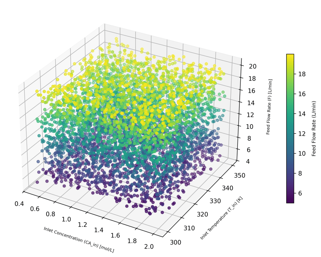
For training the AI/ML model 80% of these feature sets were selected at random and used, while for testing 20% were used as the test set. The corresponding output variables, Y, (CA_ss, T_ss) were numerically calculated for each off the 5000 input feature sets, and were used for the respective training and testing.

ML Neural Network Model

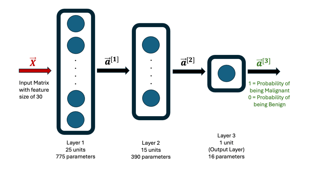
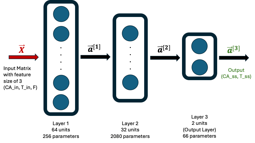
The ML model consisted of a Neural Network (NN) with 2 hidden layers and one output layer as follows. The first hidden layer had 64 neurons and the second one had 32 neurons. The final output layer had 2 neurons. The ReLU activation was used for the hidden layers and a linear activation for the output layer. The loss function used was mean-squared-error.

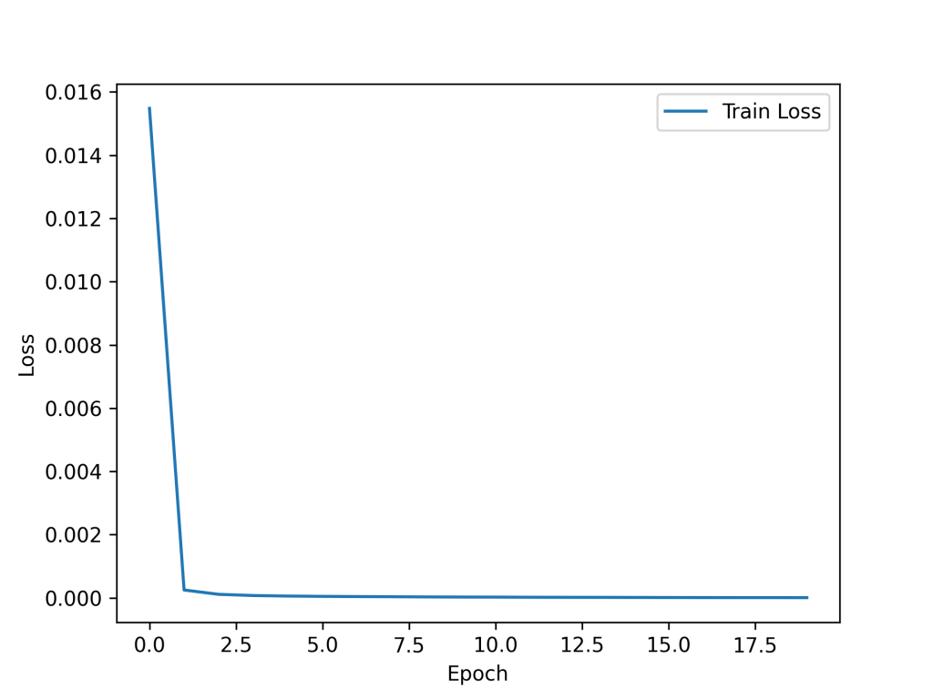
The model was trained on the training set for 20 epochs and showed rapid convergence. The loss vs epochs is presented here. The final loss was near zero (~10^-6).

After training the NN model, the Test Set was run. It yielded a Test Loss of zero (rounded off to 4 decimal places) and a Test MAE (mean average error) of 0.0025. The model has performed very nicely on the Test Set.

AI/ML Model Inference

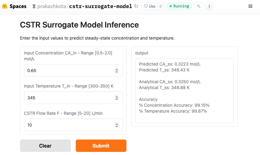
This is where AI/ML gets really exciting! I’ve packaged and deployed the neural network model on Hugging Face Spaces, using Gradio to create an interactive and web-accessible interface. Now, you can take it for a test drive—just plug in the input values, hit Submit, and watch the predictions roll in!

An actual output (screen shot) from a sample inference is shown here for input values which are within the range of the training and test sets. Both outputs (CA_ss and T_ss) are over 99% accurate.

However, this might not be all that surprising, considering the training set—comprising 4,000 feature sets (80% of 5,000)—covered a wide range of possibilities. Our result could simply be close to one of those existing data points. But what happens when we push the boundaries? My response to that would be to test a feature set where some values fall outside the training range.

For instance, in our dataset, the temperature varied between 300–350 K. What if we increase it by 10% beyond the upper limit, setting it at 385 K? Plugging this into the model, we still get an inference with over 99% accuracy! The predicted steady-state temperature (T_ss) is 385.35 K, compared to the analytical solution of 388.88 K, yielding an accuracy of 99.09%. A screenshot of the results is shared below.

Summary

I’m convinced that AI/ML has remarkable power to predict real-world scenarios with unmatched speed and accuracy. I hope this article has convinced you too. Within every company lies a hidden treasure trove of historical process data—an untapped goldmine waiting to be leveraged. When this data is extracted, cleaned, and harnessed to train a custom ML model, it transforms from an archive of past events into a powerful tool for the future.

The potential benefits are immense: vastly improved process efficiency, enhanced product quality, smarter process optimization, reduced downtime, better scheduling and planning, elimination of guesswork, and increased profitability. Incorporating ML into industrial processes requires effort—models must be carefully designed, trained, and deployed for real-time inference. While there may be cases where a single ML model can serve multiple organizations, we are still in the early stages of AI/ML adoption in process industries, and these scalable use cases are yet to be fully explored.

Right now, the opportunity is massive. The companies that act today—dusting off their historical data, building custom AI models, and integrating ML into their operations—will set the standard and lead their industries into the future. The question is: Will your company be among them?

CSTR Mathematical Model

Read this section only if you like math and want the details!

The mass and energy balance on the CSTR yield the following equations, which give the variation of concentration for the reacting species (A) and the fluid temperature (T) as a function of time (t).

$\frac{dC_A}{dt} = \frac{F}{V} (C_{A,\text{in}} - C_A) - k C_A$

$\frac{dT}{dt} = \frac{F}{V} (T_{\text{in}} - T) + \frac{-\Delta H}{\rho C_p} k C_A$

$C_A$ and $T$ are the exit concentration of A and fluid temperature $T$ . Since the residence time is long enough to reach steady state, for this irreversible reaction,

$C_A =$ CA_ss

$T =$ T_ss

The following model parameters have been taken to be a constant for all the simulated runs and analytical calculations. There is no requirement to have physical properties to be constant, since they could be allowed to vary with temperature. However, for this simulation they have been held constant.

$V =$ 100 L (tank volume)

${\Delta H} =$ -50,000 J/mol (heat of exothermic reaction)

${\rho} =$ 1 Kg/L (fluid density)

$C_p =$ 4184 J/Kg.K (fluid specific heat capacity)

The irreversible reaction for species (A) going to (B) is modeled as a first order rate equation, with the rate constant $k =$ 0.1 min^-1, and where $-r_A$ is the reaction rate (mol/L.min).

$-r_A = kC_A$

I have used a mix of SI and common units. However, when taken together in the equation, the combined units work consistently.

The analytical solution is easy to calculate and can be done by setting the time derivatives to zero and solving for the concentration and temperature. These are provided here for completeness.

CA_ss $= \frac{F C_{A,\text{in}} }{F + k V}$

T_ss = T_in – $\frac{\Delta H k C_A V}{\rho C_p F}$

To simulate the training set, we can calculate CA_ss and T_ss from the above equations. I have computed CA_ss and T_ss by solving the system of ordinary differential equations using scipy.integrate.solve_ivp, which is an adaptive-step solver in SciPy. The steady state values were taken as the dependent variable values after a lapse time of 50 minutes. These values would vary slightly from analytical values. But, they provide small variations, just like in real processes due to inherent fluctuations.

The Power of Machine Learning in Medical Diagnosis – Breast Cancer Mini Case using Neural Networks

Medical misdiagnoses continue to be a significant concern worldwide, often leading to unnecessary complications and preventable deaths. According to the World Health Organization (WHO), at least 5% of adults in the U.S. experience a diagnostic error annually. The impact on a global scale is even more alarming. Despite rapid advancements in Artificial Intelligence (AI) and Machine Learning (ML), adoption in clinical settings remains limited. Many healthcare professionals remain skeptical, with only 3% of European healthcare organizations expressing trust in AI-enabled diagnostics. This blog explores the application of Neural Networks in breast cancer detection using the Wisconsin Breast Cancer Dataset. It examines how TensorFlow based models can improve diagnostic accuracy and assesses the potential of AI-driven systems in medical practice

Have you felt rushed in a doctor’s office? Have you ever left an appointment wondering if the doctor thoroughly reviewed your blood test results and other relevant information? Have you doubted the Doctor’s opinion? You are not alone!

In a 2019 World Health Organization (WHO) article, WHO states that their research shows that at least 5% of adults in the United States experience a diagnostic error each year in outpatient settings. In a 2023 article in BMJ, the authors state that there are 2.59 million missed diagnoses in the US, accounting for 371,000 deaths and 424,000 disabilities. These numbers are for only the false negative errors. When considered on a global scale, the numbers are staggering.

Whatever may be the reason for the errors in medical diagnosis, it’s obvious that these numbers must come down. Most doctors that I have met for a professional consultation, for myself or my family members, have advised me not to ‘Google’ medical conditions. At the same time, they do not have enough of time or patience to explain the condition. I can’t blame them, considering their patient load and time constraints.

The enormous interest in AI and Machine Learning, in all walks of life, is a tool that doctors should be using daily to minimize errors in medical diagnosis. I had assumed that this is happening at a rapid pace. But I was so wrong on this. In a 2022 article in the Frontiers in Medicine, the authors conclude that from their survey of medical professionals in 39 countries, 38% had awareness of clinical AI, but that 53% lacked basic knowledge of clinical AI. Their work also revealed that 68% of doctors disagreed that AI would become a surrogate physician, but they believed that AI should assist in clinical decision making. In a 2024 online summary, it is mentioned that 42% of healthcare organizations in the European Union were currently using AI technologies for disease diagnosis, but that only 3% trusted AI-enabled decisions in disease diagnostics. These pieces of information only indicate that the adoption of AI for disease diagnosis is under suspicion by the professionals. If anything, the adoption is slow, though the advancement in AI and Machine Learning has been very rapid. There is a trust and acceptance deficit when it comes to AI/ML in medical practice. Integration of AI/ML into clinical workflows would be the next big challenge. Finally, regulatory approvals would be a barrier to AI/ML implementation in medical establishments. But these hurdles will be overcome in due time, hopefully sooner rather than later.

I like to work on small cases when confronted with big questions such as this one. I’ll share with you a case that is based on Breast Cancer. American Cancer Society estimates that Approximately 1 in 8 women in the US (13.1%) will be diagnosed with invasive breast cancer, and 1 in 43 (2.3%) will die from the disease. Breastcancer.org estimates that approximately 310,720 women are expected to be diagnosed with invasive breast cancer annually in the US. Stopbreastcancer.org estimates that the mortality rate in the US is about 42,170 annually. WHO reports that in 2022 approximately 2.3 million women worldwide were diagnosed with breast cancer, accounting for 11.6% of all cancer cases globally. Further, it reported 670,000 breast cancer related deaths in 2022.

Doctors use a variety of techniques to detect breast cancer – mammography, breast ultrasound, PET scans, DNA sequencing and biopsies. A biopsy, which is a small extraction of a physical sample for microscope analysis, is a standard investigation tool. The investigations are performed by pathologists. The output from this analysis are measurements and metrics that capture features, giving the pathologists a means to reliably diagnose whether the lesions are malignant or benign.

A reputed biopsy database, based on the fine needle aspiration technique, is the Diagnostic Wisconsin Breast Cancer Database. It contains data for 569 patient biopsies, with each data set having 30 measurement features, shown here.

id, diagnosis, radius_mean, texture_mean, perimeter_mean, area_mean, smoothness_mean, compactness_mean, concavity_mean, concave_points_mean, symmetry_mean, fractal_dimension_mean, radius_se, texture_se, perimeter_se, area_se, smoothness_se, compactness_se, concavity_se, concave_points_se, symmetry_se, fractal_dimension_se, radius_worst, texture_worst, perimeter_worst, area_worst, smoothness_worst, compactness_worst, concavity_worst, concave_points_worst, symmetry_worst, fractal_dimension_worst

The header contains 32 categories, but the first column is the patient ID and the second column is the actual diagnosis, M is for malignant and B is for benign. Excluding this header and the first 2 columns, the data is a matrix of size (569,30). With 30 pieces of input data for a single biopsy for a patient, it seems daunting for a pathologist to look at all of them, in its entirety, to diagnose whether a biopsy is cancerous or not. For example, the large input feature set for the first patient, based on actual data in the data set, is shown here to give you an idea of the volume of data to consider before a diagnosis.

842302,M,17.99,10.38,122.8,1001,0.1184,0.2776,0.3001,0.1471,0.2419,0.07871,1.095,0.9053,8.589,153.4,0.006399,0.04904,0.05373,0.01587,0.03003,0.006193,25.38,17.33,184.6,2019,0.1622,0.6656,0.7119,0.2654,0.4601,0.1189

Using this dataset, a Neural Network algorithm for Structured Machine Learning was created, using TensorFlow. The Jupyter Notebook Python code is on Github. The Neural Network consists of 3 hidden layers, the first one with 25 neurons (units), the second one with 15 neurons and the third one with 1 neuron. The first two layers use the ReLU function, while the last one uses the Sigmoid function. The architecture is shown here.

Rows 26 to 569 in the breast cancer data set were used as the Training set, while the first 25 rows were used as the Test set. The former is used to establish the weights and biases in each neuron in the network. The final output is either a 1 or 0, with 1 indicating that the data corresponds to a malignant diagnosis, while a 0 corresponds to a benign diagnosis.

After running the Neural Network code, the model was used to predict outputs for the entire Training set. Since the Training set contains the actual diagnosis (1 = M = Malignant) and (0 = B = Benign), it can be compared to the predicted output, to compute the accuracy of the Neural Network model. The model predicts a 99.26% accuracy. The predicted versus the actual output for the first 25 rows of the Training set is shown here. For the 15th row, the model predicts the outcome as 0, while the actual outcome is 1. Hence, the overall accuracy over the entire Training set is less than 100%, but still remarkable at 99.26%.

Next, the same model is used to predict the outcome for the Test set. The model has never seen this Test set before. It is equivalent to new patient data coming from the field. The prediction from the model for the Test set shows an accuracy of 100%! For comparison, the entire 26 rows of the predicted versus actual outcomes for the Test set is shown here.

These results are stunning. It emphatically shows the power of Machine Learning algorithms. For this specific case study, with a Training set of 543 patient records, it is possible to predict the cancer diagnosis for any new patient record, with an extremely high degree of accuracy.

With the number of tests that doctors ask patients to go through, hundreds of data values are generated. To make sense of all these data values, data analytics is required, rather than reliance on a cursory glance by a doctor. Neural Networks and Supervised Machine Learning are powerful AI tools that will benefit the patient today. AI can be applied to any disease diagnosis, for which raw data exists. Its adoption for reliable medical diagnosis is the need of the hour.

For those interested, the breast cancer dataset can also be analyzed using a Logistics Regression algorithm, using the Scikit-learn package. This code has also been provided on Github. The results are comparable to the Neural Network algorithm. Another small note – the TensorFlow package is one among several options available for writing Neural Networks code. Other choices are PyTorch (Meta), JAX (Google), MXNet (Apache) and CNTK (Microsoft).

You can take the Model for a test spin on the Hugging Face Platform – Breast Cancer Neural Network Prediction