Why Personalized Treatment Effects Matter: Building AI-Assisted Clinical Decision Support with a T-Learner

Part 2: Estimating Individual Treatment Effects with the T-Learner

Estimating the average effectiveness of a treatment across a patient population is an important first step in evidence-based medicine. However, physicians treat individual patients rather than populations, and the expected benefit of the same treatment may differ substantially from one patient to another. This article introduces the concept of the Individual Treatment Effect (ITE) and demonstrates how causal machine learning can be used to estimate personalized treatment benefits. Using a synthetic oncology dataset, a T‑learner architecture based on two Random Forest models is developed to estimate the expected clinical outcome under both treated and untreated scenarios for the same patient. The difference between these two predicted outcomes provides an estimate of the patient’s individualized treatment benefit and forms the basis of a prototype Clinical Decision Support (CDS) system. The article also discusses model evaluation, interpretation, limitations, and the role of AI in supporting, rather than replacing, physician decision making. Together with Part 1, this article provides a practical introduction to causal inference and individualized treatment-effect estimation for healthcare professionals, engineers, students, and data scientists interested in AI-assisted Clinical Decision Support.

From Average Patients to Individual Patients

In the previous article, we explored one of the central questions of causal inference:

Does a treatment improve outcomes, on average, across a patient population?

Using a synthetic clinical dataset, we demonstrated how treatment-selection bias and confounding can lead to misleading conclusions, and how propensity scores together with Inverse Probability Weighting (IPW) help produce a more credible estimate of the Average Treatment Effect (ATE).

The Average Treatment Effect is an important quantity for clinical research, public health, and healthcare policy because it summarizes the expected benefit of a treatment across an entire population. However, physicians rarely make treatment decisions for the “average” patient.

Every patient presents with a unique combination of age, disease stage, biomarkers, performance status, medical history, and many other clinical characteristics. Two patients with the same diagnosis may respond very differently to the same treatment. One patient may experience a substantial benefit, another only a modest improvement, a third may derive little or no benefit, while a fourth may actually be harmed by the treatment.

The physician’s question therefore changes from a population-level perspective to an individual one:

Will this treatment benefit the patient sitting in front of me?

Answering this question requires a different way of thinking. Instead of estimating a single treatment effect for an entire population, we seek to estimate the treatment effect for each individual patient. This quantity is known as the Individual Treatment Effect (ITE).

The goal of this article is to introduce the fundamental concepts behind estimating individualized treatment effects using machine learning. Building upon the synthetic dataset developed in Part 1, we will demonstrate how a T-learner constructs two predictive models, one representing treatment and the other representing no treatment, to estimate personalized treatment benefits. These estimates then become the foundation of a simple AI-assisted Clinical Decision Support (CDS)system.

As in the previous article, the objective is educational rather than clinical. The emphasis is on developing an intuitive understanding of the methodology rather than the underlying programming or mathematical details.

The Individual Treatment Effect (ITE)

In Part 1, we introduced the Average Treatment Effect (ATE), which estimates the expected benefit of a treatment across an entire patient population. While the ATE is valuable for clinical research and healthcare policy, it cannot tell us how much a particular patient is expected to benefit from the treatment.

To answer this question, we introduce the Individual Treatment Effect (ITE). Rather than estimating a single treatment effect for an entire population, the ITE estimates the treatment benefit for one specific patient based on that patient’s unique clinical characteristics.

Figure 1. Conceptual illustration of the Individual Treatment Effect (ITE). For a single patient with fixed clinical characteristics, two potential outcomes are estimated: the predicted survival probability if treated and the predicted survival probability if untreated. The estimated Individual Treatment Effect is the difference between these two predicted outcomes. In real clinical practice, only one of these outcomes is ever observed; the other remains the counterfactual.

For this demonstration, the clinical outcome of interest is the probability of surviving one year. The estimated Individual Treatment Effect is therefore defined as the difference between two predicted outcomes for the same patient: For this demonstration, the outcome of interest is the probability of surviving one year. The Individual Treatment Effect can therefore be expressed as:

Estimated ITE = Predicted Survival if Treated − Predicted Survival if Untreated

Mathematically, this is written as:

$\hat{\tau}_i = \hat{Y}_i(1) - \hat{Y}_i(0)$

where:

$\hat{Y}_i(1)$ is the estimated probability of one-year survival if patient i receives the treatment.

$\hat{Y}_i(0)$ is the estimated probability of one-year survival if patient i does not receive the treatment.

$\hat{\tau}_i$ is the estimated Individual Treatment Effect.

Figure 1 illustrates this concept. For a single patient with fixed clinical characteristics, two hypothetical outcomes are estimated, one assuming the patient receives treatment and the other assuming the patient does not. The difference between these two predicted outcomes represents the estimated Individual Treatment Effect.

An estimated ITE greater than zero suggests that the treatment is expected to improve the patient’s probability of surviving one year. An estimated ITE close to zero indicates little expected benefit, while a negative estimated ITE suggests that the treatment may not be beneficial and could potentially be associated with a poorer outcome than the alternative.

There is, however, an important distinction between this synthetic demonstration and real clinical practice. Because the dataset was deliberately engineered, the True ITE is known for every synthetic patient. This allows us to objectively evaluate how accurately our machine learning model estimates individualized treatment effects.

In real-world healthcare, the True ITE is never observed. We only observe the outcome corresponding to the treatment that was actually received. The alternative outcome, the counterfactual, remains unknown. Consequently, a Clinical Decision Support system can estimate the treatment benefit for an individual patient, but it can never know the true treatment effect with certainty. Its role is to provide evidence that supports, rather than replaces, clinical judgment.

Why Machine Learning?

The previous section introduced the concept of the Individual Treatment Effect (ITE) as the difference between two potential outcomes for the same patient. The natural question is:

How can these two outcomes be estimated?

Traditional statistical models often assume relatively simple relationships between patient characteristics and clinical outcomes. In practice, however, patient responses are influenced by many interacting factors. Age, disease stage, biomarkers, performance status, smoking history, genetics, and other clinical variables may all contribute to treatment response, often in complex and nonlinear ways.

Machine learning provides a flexible framework for learning these relationships directly from historical patient data. Rather than assuming a predetermined mathematical equation, machine learning algorithms discover patterns by analyzing large numbers of patient records. This ability to model complex interactions makes machine learning particularly attractive for estimating individualized treatment effects.

For this demonstration, we use a Random Forest Regressor, although many other machine learning algorithms could also be employed. The objective is not to identify the “best” machine learning model, but to demonstrate the fundamental concept of personalized treatment-effect estimation. The methodology described in this article is therefore independent of the specific machine learning algorithm.

The key idea is surprisingly simple. Instead of building a single predictive model for all patients, we build two separate models:

one model learns from patients who received the treatment, and
a second model learns from patients who did not receive the treatment.

Each model estimates the probability of one-year survival under its respective treatment condition. For any individual patient, both models can then be used to estimate the two potential outcomes required to calculate the Individual Treatment Effect.

This approach forms the basis of the T-learner, one of the simplest and most intuitive methods for estimating individualized treatment effects. The next section introduces the T‑learner architecture and demonstrates how these two predictive models work together to estimate personalized treatment benefits.

The T-Learner: Estimating Individual Treatment Effects

The T-learner provides a remarkably intuitive solution to the problem introduced in the previous section: how can we estimate the two potential outcomes for the same patient? Its name is derived from the use of two independent predictive models, one for patients who received the treatment and another for patients who did not.

Unlike conventional predictive modeling, the objective of the T-learner is not merely to predict a clinical outcome. Instead, it seeks to estimate what would happen under both treatment scenarios for every individual patient.

Using the historical patient data, the T-learner first separates the dataset into two groups:

patients who received the treatment, and
patients who did not receive the treatment.

A separate machine learning model is then trained for each group. In this demonstration, both models use the Random Forest Regressor algorithm, although the methodology is equally applicable to many other machine learning algorithms.

For this synthetic dataset, the selected outcome variable (Y) is the probability of one-year survival. This outcome was intentionally chosen for educational purposes because it is intuitive and easy to interpret. In practice, however, the outcome variable can represent any clinically meaningful endpoint, depending on the application. Examples include three-year or five-year survival, disease recurrence, hospital readmission, treatment response, adverse events, quality-of-life measures, or any other outcome of interest.

The first model learns the relationship between the patient characteristics and the selected clinical outcome for patients who received treatment. The second model learns the corresponding relationship for patients who did not receive treatment. Each model therefore estimates the expected outcome under one specific treatment scenario.

In supervised machine learning, the selected clinical endpoint is commonly denoted by the outcome variable ${Y}$ . Because the true outcome is unknown for a new patient, the machine learning models estimate the predicted outcome, denoted by $\hat{Y}$ .

Once both models have been trained, a new patient can be evaluated. As introduced in Part 1, the patient’s baseline covariates, or features (X) in machine learning terminology, are presented to both models, regardless of the treatment that the patient may ultimately receive.

Figure 2. Workflow of the T-learner for estimating the Individual Treatment Effect (ITE). Historical patient data are separated into treated and untreated groups to train two independent machine learning models. For a new patient with baseline covariates (features X), both models estimate the selected clinical outcome under the treated and untreated scenarios. The difference between these two predicted outcomes, $\hat{\tau}_i = \hat{Y}_i(1) - \hat{Y}_i(0)$ , represents the estimated Individual Treatment Effect, which forms the basis of AI-assisted Clinical Decision Support.

The first model estimates the expected outcome if the patient were treated, while the second estimates the expected outcome if the same patient were untreated. The difference between these two predicted outcomes is the estimated Individual Treatment Effect. Figure 2 illustrates the workflow of the T-learner used in this study.

The important observation is that both predictions are generated for the same patient. The machine learning models are not predicting outcomes for two different patients, but rather estimating two hypothetical outcomes for one individual under two different treatment scenarios. This distinction is fundamental to personalized Clinical Decision Support.

The estimated Individual Treatment Effect then becomes a quantitative measure of the expected treatment benefit. Positive values indicate that treatment is expected to improve the patient’s probability of survival, values close to zero suggest little expected benefit, while negative values indicate that treatment may not be advantageous for that particular patient.

The T-learner therefore transforms historical observational data into individualized treatment-effect estimates, providing physicians with quantitative evidence that can support treatment decisions. Importantly, these estimates should be viewed as decision-support information rather than definitive clinical recommendations. The physician remains responsible for integrating these estimates with clinical judgment, patient preferences, medical history, and other relevant considerations before selecting the most appropriate course of treatment.

Building the Synthetic Clinical Decision Support System

The previous section introduced the T-learner as a machine learning framework for estimating Individual Treatment Effects. The next step is to apply this methodology to the synthetic dataset developed in Part 1 and construct a simple Clinical Decision Support (CDS) system.

The workflow closely follows a typical supervised machine learning pipeline. Using the historical patient dataset, the treated and untreated patient populations are first separated according to their treatment status. A Random Forest regression model is then trained independently on each group to learn the relationship between the baseline covariates (features X) and the selected clinical outcome (Y).

Once the two models have been trained, they are retained as independent predictive models. For every new patient, the same baseline covariates are supplied to both models. The treated model estimates the expected clinical outcome assuming the patient receives treatment, while the untreated model estimates the expected outcome assuming the patient does not receive treatment.

The estimated Individual Treatment Effect is then calculated as the difference between these two predicted outcomes:

$\hat{\tau}_i = \hat{Y}_i(1) - \hat{Y}_i(0)$

This estimated treatment effect forms the quantitative basis of the Clinical Decision Support recommendation.

For the purposes of this demonstration, the CDS uses a simple decision rule:

Positive estimated ITE: Treatment is expected to improve the selected clinical outcome.
Estimated ITE close to zero: Little or no expected treatment benefit.
Negative estimated ITE: Treatment may not be beneficial and should be carefully reconsidered in conjunction with other clinical information.

It is important to emphasize that this decision rule is intentionally simplified for educational purposes. Real-world Clinical Decision Support systems would incorporate many additional considerations, including confidence intervals, uncertainty estimates, treatment risks, contraindications, patient preferences, physician judgment, clinical guidelines, and cost-benefit analyses.

The objective of this synthetic demonstration is therefore not to replace clinical decision making, but to illustrate how machine learning can estimate individualized treatment benefits using historical observational data.

How Well Did the T-Learner Perform?

One advantage of using a synthetic dataset is that the True Individual Treatment Effect (True ITE) is known for every patient. This provides a unique opportunity to objectively evaluate how accurately the T-learner estimates individualized treatment effects.

In real-world clinical datasets, the True ITE is never observed because only one treatment outcome is available for each patient. Consequently, the accuracy of individualized treatment-effect estimates cannot be measured directly. Synthetic data therefore provide a valuable testing environment for understanding the strengths and limitations of personalized Clinical Decision Support systems.

To evaluate the T-learner, two commonly used regression metrics were computed:

Mean Absolute Error (MAE), which measures the average difference between the estimated and True ITE values.
Coefficient of Determination (R²), which measures how well the estimated ITE values explain the variation in the True ITE values across individual patients.

Figure 3 compares the estimated Individual Treatment Effects with the corresponding True Individual Treatment Effects for all patients in the test dataset.

Figure 3. Comparison of the True Individual Treatment Effect (True ITE) and the Estimated Individual Treatment Effect (Estimated ITE) obtained using the T-learner. Each point represents one patient in the test dataset. The dashed line represents the ideal prediction line, where the estimated treatment effect is exactly equal to the True ITE. Although considerable scatter is observed around the ideal line, reflecting the difficulty of estimating individualized treatment effects, the overall positive trend indicates that the model captures the general relationship between patient characteristics and treatment benefit.

The T-learner achieved a Mean Absolute Error (MAE) of 0.0924, indicating that, on average, the estimated Individual Treatment Effect differed from the True ITE by approximately 0.09 probability units. The model also produced an R² value of –0.8811, indicating that it did not accurately reproduce the patient-specific treatment effects observed in the synthetic dataset. Estimating Individual Treatment Effects is inherently challenging because the treatment effect is obtained as the difference between two independently predicted potential outcomes rather than from a single prediction.

At first glance, Figure 3 suggests that the T-learner struggles to accurately estimate individualized treatment effects. The broad scatter of points around the ideal prediction line and the negative coefficient of determination indicate that the model captures relatively little of the patient-to-patient variation in treatment benefit. Although the MAE remains reasonably small because the treatment effects themselves span a relatively narrow range, the negative R² highlights an important practical limitation.

The relatively poor R² observed in this demonstration emphasizes an important distinction between understanding a methodology and deploying it in clinical practice. Although the T‑learner successfully illustrates how individualized treatment effects can be estimated, the resulting model would not yet be considered sufficiently accurate for use in a real Clinical Decision Support (CDS) system. In practice, such systems require substantially stronger predictive performance, extensive external validation, calibration studies, and prospective clinical evaluation before they can be used to support physician decision making.

Nevertheless, the objective of this demonstration is educational. The synthetic dataset provides a controlled environment in which the complete causal inference workflow can be understood, from estimating potential outcomes to computing individualized treatment effects. More sophisticated causal machine learning methods, larger clinical datasets, and richer patient features would be expected to produce substantially better performance in real-world applications.

An encouraging observation nevertheless emerges when the treatment effects are averaged across the patient population. The mean True ITE was 0.0425, while the mean Estimated ITE was 0.0441. The close agreement between these two values indicates that the T-learner successfully captured the overall magnitude of the treatment benefit, even though considerable variability remained in the patient-specific estimates. This distinction is important. A model may provide useful population-level insights while still exhibiting substantial uncertainty in individual patient predictions. Improving the accuracy of individualized treatment-effect estimation remains an active area of research in causal machine learning and represents an important direction for future work.

The purpose of this demonstration is therefore not to present a clinically validated prediction model, but rather to illustrate the complete workflow for estimating individualized treatment effects and incorporating them into an AI-assisted Clinical Decision Support system.

From the T-Learner to Clinical Decision Support

The ultimate goal of estimating Individual Treatment Effects is not to produce another machine learning metric, but to assist physicians in making more informed treatment decisions. This is where the T-learner becomes the foundation of a Clinical Decision Support (CDS) system.

Consider a physician evaluating a newly diagnosed patient. The patient’s baseline covariates (features X) are entered into the CDS, either manually or automatically from the electronic health record. These features are then supplied to both T-learner models.

The treated model estimates the patient’s expected clinical outcome if the treatment is administered, while the untreated model estimates the expected outcome if treatment is withheld. The difference between these two predicted outcomes is the estimated Individual Treatment Effect.

Rather than presenting only a numerical value, a practical CDS would summarize the results in a form that is easy for clinicians to interpret. For example, the system could display the predicted outcome under both treatment scenarios, the estimated treatment benefit, and a concise explanation of how the recommendation was derived. This allows physicians to understand not only the recommendation itself, but also the reasoning behind it.

Importantly, the estimated Individual Treatment Effect should not be interpreted as a definitive recommendation to treat or not to treat. It is one piece of evidence among many that clinicians consider when making patient-care decisions. Medical history, laboratory findings, imaging studies, treatment risks, patient preferences, comorbidities, and clinical guidelines all remain essential components of the final decision.

The value of a Clinical Decision Support system lies in its ability to rapidly perform complex calculations that are impossible to carry out mentally during a patient consultation. Rather than replacing physician expertise, the system augments it by providing quantitative estimates derived from historical patient data.

The synthetic demonstration presented in this article represents a simplified proof of concept. Nevertheless, it illustrates an important principle: once individualized treatment effects can be estimated reliably, they can be incorporated into interactive software tools that provide personalized, evidence-based decision support at the point of care.

A Worked Clinical Example

The concepts presented thus far become much easier to appreciate when viewed through the lens of an individual patient. To illustrate the workflow of the T-learner within a Clinical Decision Support (CDS) system, consider the synthetic patient shown below. Although this patient is entirely computer generated, the clinical characteristics were chosen to resemble those commonly encountered in oncology practice.

Table 1. Clinical characteristics (features X) of a representative synthetic patient used to illustrate the Clinical Decision Support workflow.

Clinical Variable	Value
Age	68 years
Smoking history	35 pack-years
Disease stage	III
Performance status	1
Biomarker positive	Yes

As with any new patient, the baseline covariates (features X) are supplied simultaneously to both T-learner models. One model estimates the expected clinical outcome assuming the patient receives treatment, while the second estimates the expected outcome assuming treatment is not administered. The difference between these two predicted outcomes is the estimated Individual Treatment Effect.

For this patient, the Clinical Decision Support system produced the following estimates:

Predicted one-year survival without treatment: 15.1%
Predicted one-year survival with treatment: 38.1%
Estimated Individual Treatment Effect: 23.0 percentage points

Based on these estimates, the CDS concludes that the treatment is likely to be beneficial for this patient.

Figure 4 illustrates the deployed Clinical Decision Support application developed for this demonstration. Users specify baseline patient characteristics, including age, smoking history, disease stage, performance status, and biomarker status. The application estimates the predicted one-year survival probabilities under treatment and no-treatment scenarios, computes the Individual Treatment Effect (ITE), and presents an educational treatment recommendation. The application demonstrates how causal machine learning models can be integrated into an interactive Clinical Decision Support workflow.

The live demonstration is available at models.mlpowersai.com and is intended solely for educational purposes using synthetic patient data.

Figure 4. Interactive Clinical Decision Support (CDS) application demonstrating individualized treatment-effect estimation using the deployed T-learner model. Users enter patient characteristics, and the system estimates predicted one-year survival with and without treatment, the individualized treatment benefit, and an educational treatment recommendation.

At first glance, the recommendation appears straightforward. However, the true value of the CDS lies not in the recommendation itself, but in the quantitative evidence that supports it. Rather than simply stating that treatment is recommended, the system explains why. In this example, the model estimates that treatment increases the patient’s probability of surviving one year by approximately 23 percentage points, a difference that may be clinically meaningful.

Equally important is recognizing what the CDS does not do. It does not account for every aspect of patient care. Factors such as treatment toxicity, coexisting medical conditions, quality of life, patient preferences, cost, and physician experience remain essential components of the final clinical decision. The CDS therefore serves as an additional source of evidence, complementing rather than replacing physician judgment.

This simple example illustrates the central idea behind individualized Clinical Decision Support. Every patient enters the system with a unique set of clinical characteristics. Instead of relying solely on the average treatment benefit observed across an entire population, the CDS estimates the expected benefit for that individual patient. Although the estimates are imperfect and subject to uncertainty, they represent a meaningful step toward more personalized, data-driven medicine.

Future Direction

Although this demonstration uses a synthetic dataset, it illustrates a broader direction for the future of AI-assisted Clinical Decision Support. We only see the outcome corresponding to the treatment that was actually received, while the alternative outcome remains an unobservable counterfactual.

Despite this fundamental limitation, causal machine learning provides a practical framework for estimating individualized treatment benefits from historical observational data. The T-learner presented in this article illustrates one of the simplest approaches to addressing this problem. By independently modeling the treated and untreated patient populations, it becomes possible to estimate how a particular patient may respond under two different treatment scenarios and to quantify the expected treatment benefit.

This demonstration intentionally used a synthetic dataset with a known ground truth. Although the predictive accuracy at the individual patient level remains imperfect, the exercise provides valuable insight into how causal inference and machine learning can be combined to build Clinical Decision Support systems. More importantly, it establishes a framework that can be extended to real-world healthcare datasets using more advanced causal machine learning methods.

The examples presented in this two-part series represent an educational proof of concept rather than a clinically validated decision-support tool. Real-world implementation would require carefully curated clinical data, rigorous model validation, regulatory oversight, prospective evaluation, and close collaboration between physicians, data scientists, and healthcare organizations.

Nevertheless, the underlying vision is compelling. Instead of relying solely on population averages, future Clinical Decision Support systems will increasingly estimate treatment benefits for individual patients, helping physicians make more personalized, evidence-based decisions. Artificial intelligence will not replace clinical expertise, but it can augment it by rapidly analyzing complex patient data and providing quantitative estimates that would otherwise be impossible to calculate during a clinical consultation.

For me, this project has also been a valuable learning exercise. Building the synthetic dataset, implementing the T-learner, and critically evaluating its performance have reinforced an important lesson: successful AI in healthcare is not simply about training predictive models. It requires understanding the underlying causal questions, carefully interpreting the results, and recognizing both the strengths and limitations of the methodology.

Related Resources

This article is part of an educational series on causal machine learning and Clinical Decision Support.

Companion Article (Part 1):
Why Prediction Is Not Enough: A Practical Introduction to Causal Inference for Clinical Decision Support
Companion Article (Part 2):
Why Personalized Treatment Effects Matter: Building AI-Assisted Clinical Decision Support with a T-Learner
Live Clinical Decision Support Demonstration:
https://models.mlpowersai.com/cds-estimate.html

Call to Action

Explore the live Clinical Decision Support demonstration and discover custom Healthcare AI solutions.

The Clinical Decision Support application described in this article is now available as an interactive demonstration.

Try the live demo here

MLPowersAI develops custom machine learning and causal AI solutions for healthcare, life sciences, and process industries. We build deployment-ready applications that transform data into practical decision-support tools while maintaining scientific transparency and interpretability.

Our expertise spans predictive machine learning, causal inference, clinical decision support, digital twins, and AI agents for scientific and industrial applications.

🔗 Visit us at MLPowersAI.com
🔗 Connect via LinkedIn for discussions or collaboration inquiries.

Acknowledgement

The opening illustration was created using Google’s Flow image generation system based on a prompt developed collaboratively by the author and OpenAI’s ChatGPT. Figures 1 and 2 were created using OpenAI’s ChatGPT image generation capabilities. Figure 3 was generated programmatically from the author’s Python code within a Jupyter Notebook. Figure 4 is a screenshot of the deployed Clinical Decision Support (CDS) web application developed by the author using FastAPI and a custom HTML/CSS/JavaScript interface. The scientific concepts, figure design, interpretation, and accompanying captions were developed, reviewed, and validated by the author.

Why Prediction Is Not Enough: A Practical Introduction to Causal Inference for Clinical Decision Support

Part 1: Understanding Average Treatment Effects

Artificial Intelligence has become increasingly effective at predicting clinical outcomes, but prediction alone cannot determine whether a treatment actually caused an observed benefit. This distinction between prediction and causation lies at the heart of modern Clinical Decision Support (CDS). This article introduces the fundamental concepts of causal inference using a synthetic clinical dataset developed for educational purposes. Through practical examples, it explains counterfactuals, treatment-selection bias, confounding, propensity scores, and Inverse Probability Weighting (IPW), illustrating how these methods improve estimation of the Average Treatment Effect (ATE). Rather than emphasizing programming or mathematical detail, the focus is on developing an intuitive understanding of why causal inference matters and how it forms the foundation for personalized, AI-assisted clinical decision making. This article is the first in a two-part series that progresses from causal inference to individualized treatment recommendations and practical Clinical Decision Support systems.

The Physician’s Question

Imagine a physician treating a patient recently diagnosed with cancer.

Several treatment options may be available. One treatment may improve the patient’s chance of surviving the next year, while another may offer little benefit or expose the patient to unnecessary side effects. Naturally, the physician wants to answer a simple but important question:

Will this treatment actually benefit this patient?

At first glance, the answer appears straightforward. We could compare the one-year survival of patients who received the treatment with those who did not. If the treated patients had better survival, we might conclude that the treatment works.

Unfortunately, real-world medicine is rarely that simple.

Patients who receive a treatment are often fundamentally different from those who do not. They may differ in age, disease stage, performance status, genetic biomarkers, smoking history, or many other clinical characteristics. Physicians make treatment decisions based on these factors every day, and rightly so. Consequently, the treated and untreated groups are rarely directly comparable.

This raises an important question:

Did the treatment improve survival, or were the treated patients simply different to begin with?

That question is much more difficult than it first appears. It requires us to separate the effect of the treatment itself from the differences that already existed between the two groups of patients. This is the central challenge of causal inference.

In this article, I introduce the fundamental ideas behind causal inference using a synthetic clinical dataset developed for educational purposes. We will see why simple comparisons can be misleading, how propensity scores and inverse probability weighting (IPW) help create more comparable treatment groups, and how these methods provide a more credible estimate of the Average Treatment Effect (ATE).

In the second article of this series, we will build upon these ideas to estimate treatment benefits for individual patients using a T-learner, illustrating how modern AI techniques can support personalized Clinical Decision Support (CDS).

Prediction Is Not Causation

Imagine Modern machine learning has become remarkably good at making predictions. Given sufficient historical data, a model can estimate the probability that a patient will survive, develop a complication, or respond to a particular therapy. These predictions can be valuable, but they do not necessarily tell us whether a treatment caused the observed outcome.

To appreciate the difference, consider two related but fundamentally different questions.

Prediction: What is likely to happen?
Causation: What would happen if we changed the treatment decision?

The first question looks only at the future outcome. The second asks how the outcome would change under an alternative course of action.

This distinction is subtle but important.

Suppose historical data show that patients receiving a particular treatment have higher one-year survival than patients who do not receive it. It may be tempting to conclude that the treatment improved survival. However, the treated patients may have been younger, diagnosed earlier, or possessed favorable genetic biomarkers. Their better outcomes may have been due, at least in part, to these underlying characteristics rather than the treatment itself.

In other words, correlation does not necessarily imply causation.

This challenge is not unique to medicine. Engineers, economists, and business analysts face the same problem whenever they attempt to estimate the effect of an intervention using observational data. The central question becomes:

How can we isolate the effect of the treatment itself from all the other factors that influence the outcome?

Answering that question is the goal of causal inference.

In the following sections, we will build a simple synthetic clinical dataset that allows us to explore these ideas in a controlled environment. Because the underlying truth is known, we can objectively evaluate how well different causal inference techniques recover the actual treatment effect.

The Counterfactual: The Outcome We Never Observe

At the heart of causal inference lies a deceptively simple idea known as the counterfactual.

Suppose a physician decides to treat a patient. One year later, the patient survives. An obvious question follows:

Did the treatment cause the patient to survive?

Unfortunately, we can never answer that question with certainty for that individual patient.

Why?

Because we only observe one version of reality.

If the patient received the treatment, we observe the outcome with treatment. We never observe what would have happened without treatment. Conversely, if the patient did not receive the treatment, we observe the outcome without treatment, but we never know what the outcome would have been had the treatment been given.

These two potential outcomes are often represented as:

Y(1) : Outcome if the patient receives treatment.
Y(0) : Outcome if the patient does not receive treatment.

For any individual patient, only one of these outcomes can ever be observed. The other remains hypothetical, it is the counterfactual (Figure 1).

This is known as the Fundamental Problem of Causal Inference. Since one of the two potential outcomes is always missing, the true treatment effect for an individual patient can never be observed directly.

Fortunately, although the true treatment effect for an individual patient is unknowable, it is still possible to estimate treatment effects across a population using carefully designed statistical methods. These methods attempt to compare patients who are as similar as possible, differing primarily in whether they received the treatment.

This is precisely where causal inference differs from conventional predictive machine learning. Rather than simply predicting an outcome, it attempts to estimate what might have happened under an alternative treatment decision.

Figure 1: The counterfactual problem. For each patient, we can observe only one of the two potential outcomes (with treatment Y(1) or without treatment Y(0)). The other outcome remains unobserved, which is the counterfactual.

In the next section, we will construct a synthetic clinical dataset that allows us to simulate both potential outcomes. Because we control how the data are generated, we know the underlying treatment effects exactly. This provides an ideal environment for understanding how causal inference methods work before applying them to real-world clinical data.

Why Use Synthetic Data?

One of the greatest challenges in developing and evaluating causal inference methods is that the true treatment effect for an individual patient is fundamentally unknowable. We observe only one of the two possible outcomes, the one corresponding to the treatment that was actually received. The counterfactual outcome remains forever unobserved.

This creates an important practical problem. If the true treatment effect is never known, how can we determine whether a causal inference method is producing accurate estimates?

One solution is to construct a synthetic dataset in which the underlying relationships are deliberately engineered by the investigator. Unlike real clinical data, where the truth is hidden, synthetic data allow us to define the treatment assignment mechanism, the survival probabilities, and the true treatment effect for every individual patient.

For this article, I developed a synthetic clinical dataset representing 5,000 fictional patients diagnosed with a hypothetical disease that I refer to as Cancer-X. The disease itself is fictional and serves only as an educational example. The objective is not to model a specific cancer, but to create a realistic environment for demonstrating the fundamental concepts of causal inference and Clinical Decision Support.

Each patient is characterized by several baseline clinical features, including age, smoking history, disease stage, performance status, and biomarker status. These variables influence both the probability of receiving treatment and the patient’s expected survival. By carefully controlling these relationships, we can introduce realistic treatment-selection bias, evaluate causal inference methods, and compare their estimates with the known ground truth.

This ability to compare an estimated treatment effect with the true underlying treatment effect is one of the greatest advantages of synthetic data. It transforms an otherwise impossible validation problem into a controlled scientific experiment.

Engineering a Realistic Dataset

The synthetic dataset was designed to resemble a realistic clinical decision-making environment rather than to model any specific disease. The objective was to create a patient population in which physicians would reasonably make different treatment decisions based on each patient’s clinical characteristics.

Five baseline variables were selected to describe each patient:

Age (years)
Smoking history (pack-years)
Disease stage (1–4)
Performance status (0–3)
Biomarker status (positive or negative)

These variables are commonly referred to as baseline covariates because they are measured before the treatment decision is made. In real clinical practice, physicians routinely consider these and many other factors when deciding whether a patient should receive a particular therapy. The baseline covariates are also known as features (X) in machine learning.

The values assigned to these variables were generated to resemble realistic patient populations while remaining entirely synthetic. The precise probability distributions are not important for understanding the concepts presented in this article. What is important is that the variables exhibit sufficient diversity to create meaningful differences among patients.

The next step was to model how treatment decisions are made.

As a result, the synthetic dataset intentionally contains treatment-selection bias. The treated and untreated groups differ systematically before treatment is even evaluated. For example, patients with more advanced disease or favorable biomarkers were more likely to receive treatment, while patients with poorer performance status were somewhat less likely to be treated. This phenomenon is known as confounding and is one of the principal reasons why simple comparisons between the two groups can produce biased estimates of the Average Treatment Effect (ATE).

This intentional treatment-selection bias is known as confounding. It creates systematic differences between the treated and untreated groups, making a simple comparison of their outcomes potentially misleading.

Finally, the synthetic dataset was engineered so that treatment genuinely improves survival for some patients more than others. Consequently, each patient possesses an underlying true individual treatment effect, although this quantity is known only because the data are simulated. In real clinical datasets, the true treatment effect for an individual patient can never be observed directly.

By controlling both the treatment assignment process and the underlying treatment effects, the synthetic dataset becomes a valuable laboratory for studying causal inference methods under conditions that resemble real-world clinical practice.

A Naive Comparison of the Two Groups

Suppose we momentarily ignore the treatment-selection bias built into our synthetic dataset and simply compare the one-year survival of the treated and untreated patients. This approach is known as the naive estimate of the Average Treatment Effect (ATE). It assumes that the only meaningful difference between the two groups is whether they received the treatment.

The naive ATE is calculated simply as:

Naive ATE = (Average survival of treated patients − Average survival of untreated patients)

Applying this calculation to the synthetic dataset produced the following result (Table 1):

Table 1. ATE Values from Dataset Simulation.

Estimate	Value
Naive ATE	3.40%
True ATE	4.40%

At first glance, the treatment appears to improve one-year survival by 3.4 percentage points. However, because we engineered the synthetic dataset, we know that the true Average Treatment Effect is actually 4.4 percentage points. The discrepancy is not caused by an error in the calculation. The arithmetic is perfectly correct.

Rather, the naive comparison is biased because the treated and untreated groups were systematically different before treatment was ever administered. Patients with different disease stages, biomarker status, and performance status were not equally likely to receive treatment. Consequently, part of the observed difference in survival reflects differences in the patient populations rather than the effect of the treatment itself (Figure 2).

Figure 2: A naive comparison of one-year survival between the treated and untreated patient groups. The observed difference in mean survival (31.2% vs. 27.8%) suggests an Average Treatment Effect (ATE) of 3.4%. However, because the two groups differ systematically in their baseline characteristics, this naïve estimate is biased and does not represent the true causal effect of the treatment.

The important lesson is that a simple comparison between treated and untreated patients does not necessarily estimate the causal effect of the treatment. It estimates the combined influence of the treatment and the differences that already existed between the two groups.

This is precisely the problem that causal inference seeks to solve.

Propensity Scores: Making the Groups Comparable

The naive comparison presented in the previous section is biased because the treated and untreated patients are fundamentally different before treatment is even administered. To estimate the causal effect of the treatment, we first need to account for these differences.

One elegant solution is the propensity score (Figure 3).

Figure 3: The propensity score is the estimated probability that a patient receives treatment based on baseline covariates. It predicts treatment assignment rather than clinical outcome and serves as the basis for Inverse Probability Weighting (IPW).

The propensity score is defined as the probability that a patient receives treatment based solely on the patient’s baseline characteristics (covariates). In our synthetic dataset, these covariates include age, smoking history, disease stage, performance status, and biomarker status.

Conceptually, the propensity score answers the following question:

Given this patient’s characteristics, how likely is the physician to recommend treatment?

Notice that the propensity score does not estimate whether the patient will survive. Nor does it estimate whether the treatment is effective. It estimates only the probability of receiving treatment.

Patients with similar propensity scores have similar baseline characteristics, even if one patient received treatment and the other did not. This provides a common basis for comparing patients who are otherwise clinically alike.

To estimate the propensity score, I trained a logistic regression model using only the baseline covariates. The model predicts the probability of treatment assignment for every patient in the synthetic dataset.

Figure 4: Distribution of the estimated propensity scores for treated and untreated patients in the synthetic dataset. Each patient’s propensity score represents the estimated probability of receiving treatment based on the baseline covariates. Although the two distributions overlap substantially, they are not identical, reflecting the treatment-selection bias intentionally introduced into the dataset. These propensity scores form the basis for Inverse Probability Weighting (IPW).

The overlap between the two distributions is particularly important. It indicates that patients with similar baseline characteristics exist in both the treated and untreated groups, making meaningful causal comparisons possible after appropriate statistical adjustment.

The resulting propensity scores range between 0 and 1. Patients with values close to 1 were highly likely to receive treatment based on their clinical characteristics, whereas patients with values close to 0 were unlikely to be treated.

The propensity score itself does not remove bias. Rather, it provides a quantitative measure of how likely each patient was to receive treatment. In the next section, we will use these propensity scores to rebalance the treated and untreated groups through Inverse Probability Weighting (IPW).

Inverse Probability Weighting (IPW): Rebalancing the Patient Population

The propensity score tells us how likely each patient was to receive treatment based on their baseline characteristics. However, knowing these probabilities alone does not remove the treatment-selection bias.

The next question is:

How can we use the propensity scores to create a fairer comparison between the treated and untreated groups?

One elegant solution is Inverse Probability Weighting (IPW).

The basic idea is surprisingly intuitive. Patients who received the treatment despite being unlikely to receive it provide particularly valuable information. Likewise, untreated patients who were highly likely to receive treatment are also informative because they represent patients who are relatively uncommon within their respective groups.

IPW assigns a statistical weight to every patient based on the inverse of the patient’s propensity score.

Patients who were very likely to receive the treatment receive relatively small weights because many similar patients already exist in the dataset. In contrast, patients who were unlikely to receive the treatment receive larger weights because they are comparatively rare and therefore have greater influence in the weighted analysis.

Rather than changing the patients themselves, IPW changes how much influence each patient has when estimating the Average Treatment Effect (ATE). In effect, it creates a weighted pseudo-population in which the treated and untreated groups become much more comparable with respect to their baseline characteristics.

The goal is not to eliminate all differences between patients. Rather, it is to reduce the systematic differences that arose from the treatment-selection process. By making the two groups more similar before comparing their outcomes, IPW produces a more credible estimate of the causal effect of the treatment.

Figure 5: Conceptual illustration of Inverse Probability Weighting (IPW). Rather than changing the patients in the dataset, IPW assigns different statistical weights to individual patients based on their propensity scores, creating a weighted pseudo-population in which the treated and untreated groups become more comparable. This reduces bias due to treatment-selection and confounding when estimating the Average Treatment Effect (ATE).

This improvement can be seen by comparing the baseline characteristics of the treated and untreated patient groups before and after applying IPW.

Table 2. Comparison of mean baseline covariates between the treated and untreated patient groups before Inverse Probability Weighting (IPW). The observed differences illustrate the presence of treatment-selection bias and confounding in the synthetic dataset.

Mean Values	Age	Smoking History	Stage	Performance Status	Biomarker Positive
Untreated	64.76	30.06	2.65	1.26	32.4%
Treated	66.27	30.85	3.11	0.89	43.3%
Difference	1.51	0.80	0.45	-0.37	10.90%

Before weighting, the treated and untreated groups differ noticeably in age, disease stage, performance status, and biomarker status (Table 2). These differences reflect the treatment-selection bias intentionally engineered into the synthetic dataset. Consequently, a direct comparison of outcomes between the two groups is likely to produce a biased estimate of the treatment effect.

Table 3. Comparison of mean baseline covariates between the treated and untreated patient groups after Inverse Probability Weighting (IPW). The substantially reduced differences demonstrate improved covariate balance, creating treatment groups that are more comparable for estimating the Average Treatment Effect (ATE).

Mean Values	Age	Smoking History	Stage	Performance Status	Biomarker Positive
Untreated	65.03	30.21	2.74	1.19	34.3%
Treated	64.94	29.99	2.71	1.15	33.1%
Difference	-0.09	-0.22	-0.03	-0.03	-1.2%

After applying IPW, the differences between the two groups become substantially smaller (Table 3). Although the original patient data remain unchanged, the statistical weighting creates a pseudo-population in which the treated and untreated groups are much better balanced with respect to their measured baseline covariates. This improved covariate balance forms the basis for a more credible causal comparison.

Having created more comparable treatment groups, we can now re-estimate the Average Treatment Effect (Table 4).

Table 4. Average Treatment Effect across Techniques

Estimate	Value
Naive ATE	3.4%
IPW ATE	4.9%
True ATE	4.4%

The IPW estimate is noticeably closer to the true Average Treatment Effect than the naive estimate. This illustrates the primary purpose of IPW: not to guarantee the correct answer, but to reduce bias arising from treatment-selection and confounding by creating treatment groups that are more comparable.

Estimating the Average Treatment Effect

The results presented in Table 4 illustrate the impact of adjusting for treatment-selection bias using Inverse Probability Weighting (IPW).

The naive comparison estimated a treatment benefit of 3.4 percentage points, whereas the IPW-adjusted analysis estimated a treatment benefit of 4.9 percentage points. Because the synthetic dataset was engineered with a known true Average Treatment Effect of 4.4 percentage points, we are able to compare both estimates with the underlying ground truth.

The naive estimate underestimates the true treatment effect because the treated and untreated groups were systematically different before treatment was administered. Patients were not assigned treatment at random; treatment decisions depended on their baseline clinical characteristics. Consequently, a simple comparison between the two groups cannot isolate the causal effect of the treatment.

After applying IPW, the estimated treatment effect moves substantially closer to the known true value. This does not imply that IPW always produces the correct answer. Rather, it demonstrates how reducing treatment-selection bias through improved covariate balance can produce a more credible estimate of the causal effect.

One of the greatest advantages of this synthetic experiment is that the true treatment effect is known because the dataset was synthetically generated. This allows us to objectively evaluate the performance of different causal inference methods. In real-world observational studies, the true Average Treatment Effect is generally unknown, making such direct validation impossible.

The goal of causal inference is therefore not to eliminate uncertainty, but to make treatment-effect estimates more reliable by accounting for systematic differences between the groups being compared.

Limitations of This Demonstration

Although the synthetic experiment illustrates the fundamental concepts of causal inference, it is important to recognize its limitations. The objective of this demonstration is educational, to explain the fundamental concepts of causal inference using a controlled synthetic dataset, rather than to develop or validate a clinical decision support system.

First, the dataset is entirely synthetic. The relationships between the patient characteristics, treatment assignment, and clinical outcomes were deliberately engineered to create a controlled learning environment. While the variables and treatment-selection process resemble real clinical decision making, they do not represent any specific disease or patient population.

Second, the synthetic dataset assumes that all important patient characteristics influencing treatment assignment have been measured. In real-world clinical practice, this assumption is rarely satisfied. Important factors such as physician judgment, patient preferences, socioeconomic status, genetic information, or unrecorded clinical observations may also influence treatment decisions. These unmeasured confounders remain one of the greatest challenges in causal inference.

Third, propensity score methods, including Inverse Probability Weighting (IPW), estimate population-level treatment effects. They answer questions such as:

Does the treatment improve outcomes on average across the patient population?

They do not answer a physician’s most important question:

Will this treatment benefit the individual patient sitting in front of me?

Finally, although IPW reduced the bias in this synthetic experiment, it did not perfectly recover the true Average Treatment Effect. Statistical adjustment improves the credibility of the estimate, but it does not eliminate uncertainty. Like all statistical models, causal inference methods depend on the quality of the available data and the validity of their underlying assumptions.

These limitations should not be viewed as weaknesses of causal inference. Rather, they reflect the inherent difficulty of estimating treatment effects from observational data. The goal is not perfect certainty, but better-informed decision making through principled statistical methods.

Looking Ahead: From Population Averages to Personalized Treatment Decisions

Throughout this article, we have focused on estimating the Average Treatment Effect (ATE), the expected benefit of a treatment across an entire patient population. Causal inference methods such as propensity scores and Inverse Probability Weighting (IPW) help reduce treatment-selection bias and produce more credible estimates of these population‑level effects.

These methods answer an important scientific question:

Does the treatment work, on average?

However, physicians rarely treat the “average” patient.

Every patient is unique, with a distinct combination of age, disease stage, performance status, biomarkers, medical history, and many other clinical characteristics. The question facing the physician is therefore much more personal:

Will this treatment benefit the individual patient sitting in front of me?

Answering that question requires estimating an Individual Treatment Effect (ITE) rather than a single average treatment effect across the population. Unlike the ATE, which summarizes the average benefit, the ITE attempts to estimate how much a particular patient is expected to benefit from the treatment compared with the alternative of not receiving it.

Modern machine learning provides powerful tools for estimating these individualized treatment effects. One such approach is the T-learner, which builds separate predictive models for treated and untreated patients and estimates the treatment benefit for each individual by comparing the predicted outcomes under the two treatment scenarios.

In the next article, we will build upon the causal inference concepts introduced here to develop a simple AI-assisted Clinical Decision Support (CDS) system based on the T-learner. Although the demonstration will again use synthetic data, it will illustrate how causal inference and machine learning can be combined to estimate personalized treatment benefits and support more informed clinical decision making.

Ultimately, Clinical Decision Support is not about replacing physicians. It is about providing them with better quantitative evidence to complement their clinical expertise. The physician remains the final decision maker, but AI can assist by analyzing complex relationships and estimating treatment effects that are impossible to calculate mentally during routine clinical practice.

Related Resources

This article is part of an educational series on causal machine learning and Clinical Decision Support.

Companion Article (Part 1):
Why Prediction Is Not Enough: A Practical Introduction to Causal Inference for Clinical Decision Support
Companion Article (Part 2):
Why Personalized Treatment Effects Matter: Building AI-Assisted Clinical Decision Support with a T-Learner
Live Clinical Decision Support Demonstration:
https://models.mlpowersai.com/cds-estimate.html

Call to Action

Explore the live Clinical Decision Support demonstration and discover custom Healthcare AI solutions.

The Clinical Decision Support application described in this article is now available as an interactive demonstration.

Try the live demo here

Our expertise spans predictive machine learning, causal inference, clinical decision support, digital twins, and AI agents for scientific and industrial applications.

🔗 Visit us at MLPowersAI.com
🔗 Connect via LinkedIn for discussions or collaboration inquiries.

Acknowledgement

The opening illustration and Figures 1, 2, 3, and 5 were created using OpenAI’s ChatGPT image generation capabilities. Figure 4 was generated programmatically from the author’s Python code within a Jupyter Notebook. The concepts, figure design, interpretation, and accompanying captions were developed, reviewed, and validated by the author.

The Power of Machine Learning in Medical Diagnosis – Breast Cancer Mini Case using Neural Networks

Medical misdiagnoses continue to be a significant concern worldwide, often leading to unnecessary complications and preventable deaths. According to the World Health Organization (WHO), at least 5% of adults in the U.S. experience a diagnostic error annually. The impact on a global scale is even more alarming. Despite rapid advancements in Artificial Intelligence (AI) and Machine Learning (ML), adoption in clinical settings remains limited. Many healthcare professionals remain skeptical, with only 3% of European healthcare organizations expressing trust in AI-enabled diagnostics. This blog explores the application of Neural Networks in breast cancer detection using the Wisconsin Breast Cancer Dataset. It examines how TensorFlow based models can improve diagnostic accuracy and assesses the potential of AI-driven systems in medical practice

Have you felt rushed in a doctor’s office? Have you ever left an appointment wondering if the doctor thoroughly reviewed your blood test results and other relevant information? Have you doubted the Doctor’s opinion? You are not alone!

In a 2019 World Health Organization (WHO) article, WHO states that their research shows that at least 5% of adults in the United States experience a diagnostic error each year in outpatient settings. In a 2023 article in BMJ, the authors state that there are 2.59 million missed diagnoses in the US, accounting for 371,000 deaths and 424,000 disabilities. These numbers are for only the false negative errors. When considered on a global scale, the numbers are staggering.

Whatever may be the reason for the errors in medical diagnosis, it’s obvious that these numbers must come down. Most doctors that I have met for a professional consultation, for myself or my family members, have advised me not to ‘Google’ medical conditions. At the same time, they do not have enough of time or patience to explain the condition. I can’t blame them, considering their patient load and time constraints.

The enormous interest in AI and Machine Learning, in all walks of life, is a tool that doctors should be using daily to minimize errors in medical diagnosis. I had assumed that this is happening at a rapid pace. But I was so wrong on this. In a 2022 article in the Frontiers in Medicine, the authors conclude that from their survey of medical professionals in 39 countries, 38% had awareness of clinical AI, but that 53% lacked basic knowledge of clinical AI. Their work also revealed that 68% of doctors disagreed that AI would become a surrogate physician, but they believed that AI should assist in clinical decision making. In a 2024 online summary, it is mentioned that 42% of healthcare organizations in the European Union were currently using AI technologies for disease diagnosis, but that only 3% trusted AI-enabled decisions in disease diagnostics. These pieces of information only indicate that the adoption of AI for disease diagnosis is under suspicion by the professionals. If anything, the adoption is slow, though the advancement in AI and Machine Learning has been very rapid. There is a trust and acceptance deficit when it comes to AI/ML in medical practice. Integration of AI/ML into clinical workflows would be the next big challenge. Finally, regulatory approvals would be a barrier to AI/ML implementation in medical establishments. But these hurdles will be overcome in due time, hopefully sooner rather than later.

I like to work on small cases when confronted with big questions such as this one. I’ll share with you a case that is based on Breast Cancer. American Cancer Society estimates that Approximately 1 in 8 women in the US (13.1%) will be diagnosed with invasive breast cancer, and 1 in 43 (2.3%) will die from the disease. Breastcancer.org estimates that approximately 310,720 women are expected to be diagnosed with invasive breast cancer annually in the US. Stopbreastcancer.org estimates that the mortality rate in the US is about 42,170 annually. WHO reports that in 2022 approximately 2.3 million women worldwide were diagnosed with breast cancer, accounting for 11.6% of all cancer cases globally. Further, it reported 670,000 breast cancer related deaths in 2022.

Doctors use a variety of techniques to detect breast cancer – mammography, breast ultrasound, PET scans, DNA sequencing and biopsies. A biopsy, which is a small extraction of a physical sample for microscope analysis, is a standard investigation tool. The investigations are performed by pathologists. The output from this analysis are measurements and metrics that capture features, giving the pathologists a means to reliably diagnose whether the lesions are malignant or benign.

A reputed biopsy database, based on the fine needle aspiration technique, is the Diagnostic Wisconsin Breast Cancer Database. It contains data for 569 patient biopsies, with each data set having 30 measurement features, shown here.

id, diagnosis, radius_mean, texture_mean, perimeter_mean, area_mean, smoothness_mean, compactness_mean, concavity_mean, concave_points_mean, symmetry_mean, fractal_dimension_mean, radius_se, texture_se, perimeter_se, area_se, smoothness_se, compactness_se, concavity_se, concave_points_se, symmetry_se, fractal_dimension_se, radius_worst, texture_worst, perimeter_worst, area_worst, smoothness_worst, compactness_worst, concavity_worst, concave_points_worst, symmetry_worst, fractal_dimension_worst

The header contains 32 categories, but the first column is the patient ID and the second column is the actual diagnosis, M is for malignant and B is for benign. Excluding this header and the first 2 columns, the data is a matrix of size (569,30). With 30 pieces of input data for a single biopsy for a patient, it seems daunting for a pathologist to look at all of them, in its entirety, to diagnose whether a biopsy is cancerous or not. For example, the large input feature set for the first patient, based on actual data in the data set, is shown here to give you an idea of the volume of data to consider before a diagnosis.

842302,M,17.99,10.38,122.8,1001,0.1184,0.2776,0.3001,0.1471,0.2419,0.07871,1.095,0.9053,8.589,153.4,0.006399,0.04904,0.05373,0.01587,0.03003,0.006193,25.38,17.33,184.6,2019,0.1622,0.6656,0.7119,0.2654,0.4601,0.1189

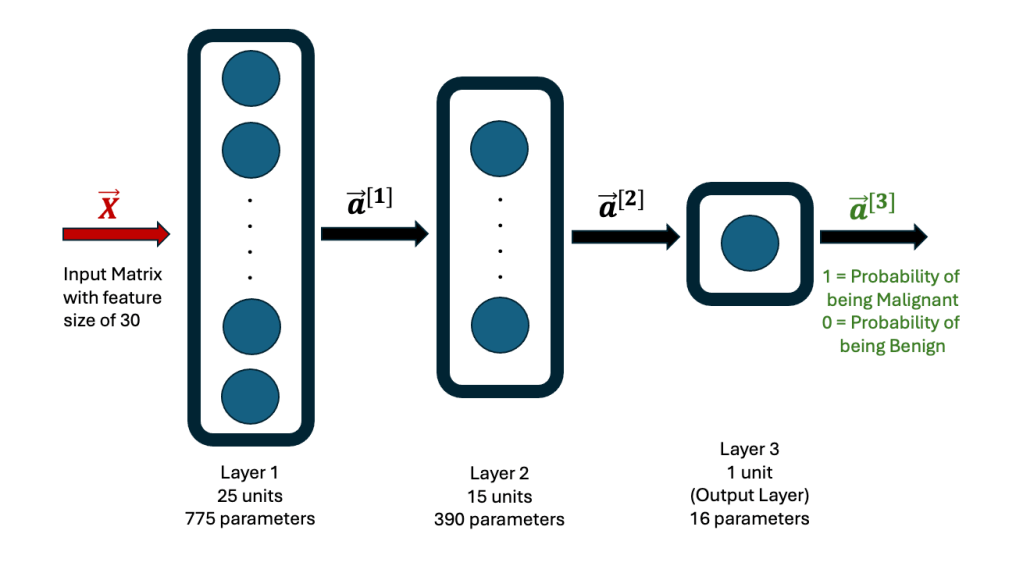
Using this dataset, a Neural Network algorithm for Structured Machine Learning was created, using TensorFlow. The Jupyter Notebook Python code is on Github. The Neural Network consists of 3 hidden layers, the first one with 25 neurons (units), the second one with 15 neurons and the third one with 1 neuron. The first two layers use the ReLU function, while the last one uses the Sigmoid function. The architecture is shown here.

Rows 26 to 569 in the breast cancer data set were used as the Training set, while the first 25 rows were used as the Test set. The former is used to establish the weights and biases in each neuron in the network. The final output is either a 1 or 0, with 1 indicating that the data corresponds to a malignant diagnosis, while a 0 corresponds to a benign diagnosis.

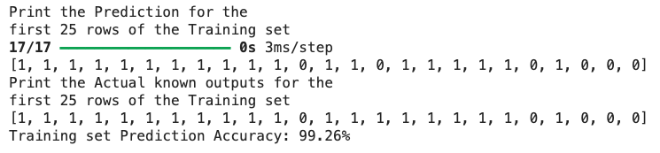
After running the Neural Network code, the model was used to predict outputs for the entire Training set. Since the Training set contains the actual diagnosis (1 = M = Malignant) and (0 = B = Benign), it can be compared to the predicted output, to compute the accuracy of the Neural Network model. The model predicts a 99.26% accuracy. The predicted versus the actual output for the first 25 rows of the Training set is shown here. For the 15th row, the model predicts the outcome as 0, while the actual outcome is 1. Hence, the overall accuracy over the entire Training set is less than 100%, but still remarkable at 99.26%.

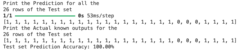
Next, the same model is used to predict the outcome for the Test set. The model has never seen this Test set before. It is equivalent to new patient data coming from the field. The prediction from the model for the Test set shows an accuracy of 100%! For comparison, the entire 26 rows of the predicted versus actual outcomes for the Test set is shown here.

These results are stunning. It emphatically shows the power of Machine Learning algorithms. For this specific case study, with a Training set of 543 patient records, it is possible to predict the cancer diagnosis for any new patient record, with an extremely high degree of accuracy.

With the number of tests that doctors ask patients to go through, hundreds of data values are generated. To make sense of all these data values, data analytics is required, rather than reliance on a cursory glance by a doctor. Neural Networks and Supervised Machine Learning are powerful AI tools that will benefit the patient today. AI can be applied to any disease diagnosis, for which raw data exists. Its adoption for reliable medical diagnosis is the need of the hour.

For those interested, the breast cancer dataset can also be analyzed using a Logistics Regression algorithm, using the Scikit-learn package. This code has also been provided on Github. The results are comparable to the Neural Network algorithm. Another small note – the TensorFlow package is one among several options available for writing Neural Networks code. Other choices are PyTorch (Meta), JAX (Google), MXNet (Apache) and CNTK (Microsoft).

You can take the Model for a test spin on the Hugging Face Platform – Breast Cancer Neural Network Prediction