Why Personalized Treatment Effects Matter: Building AI-Assisted Clinical Decision Support with a T-Learner

Part 2: Estimating Individual Treatment Effects with the T-Learner

Estimating the average effectiveness of a treatment across a patient population is an important first step in evidence-based medicine. However, physicians treat individual patients rather than populations, and the expected benefit of the same treatment may differ substantially from one patient to another. This article introduces the concept of the Individual Treatment Effect (ITE) and demonstrates how causal machine learning can be used to estimate personalized treatment benefits. Using a synthetic oncology dataset, a T‑learner architecture based on two Random Forest models is developed to estimate the expected clinical outcome under both treated and untreated scenarios for the same patient. The difference between these two predicted outcomes provides an estimate of the patient’s individualized treatment benefit and forms the basis of a prototype Clinical Decision Support (CDS) system. The article also discusses model evaluation, interpretation, limitations, and the role of AI in supporting, rather than replacing, physician decision making. Together with Part 1, this article provides a practical introduction to causal inference and individualized treatment-effect estimation for healthcare professionals, engineers, students, and data scientists interested in AI-assisted Clinical Decision Support.

From Average Patients to Individual Patients

In the previous article, we explored one of the central questions of causal inference:

Does a treatment improve outcomes, on average, across a patient population?

Using a synthetic clinical dataset, we demonstrated how treatment-selection bias and confounding can lead to misleading conclusions, and how propensity scores together with Inverse Probability Weighting (IPW) help produce a more credible estimate of the Average Treatment Effect (ATE).

The Average Treatment Effect is an important quantity for clinical research, public health, and healthcare policy because it summarizes the expected benefit of a treatment across an entire population. However, physicians rarely make treatment decisions for the “average” patient.

Every patient presents with a unique combination of age, disease stage, biomarkers, performance status, medical history, and many other clinical characteristics. Two patients with the same diagnosis may respond very differently to the same treatment. One patient may experience a substantial benefit, another only a modest improvement, a third may derive little or no benefit, while a fourth may actually be harmed by the treatment.

The physician’s question therefore changes from a population-level perspective to an individual one:

Will this treatment benefit the patient sitting in front of me?

Answering this question requires a different way of thinking. Instead of estimating a single treatment effect for an entire population, we seek to estimate the treatment effect for each individual patient. This quantity is known as the Individual Treatment Effect (ITE).

The goal of this article is to introduce the fundamental concepts behind estimating individualized treatment effects using machine learning. Building upon the synthetic dataset developed in Part 1, we will demonstrate how a T-learner constructs two predictive models, one representing treatment and the other representing no treatment, to estimate personalized treatment benefits. These estimates then become the foundation of a simple AI-assisted Clinical Decision Support (CDS)system.

As in the previous article, the objective is educational rather than clinical. The emphasis is on developing an intuitive understanding of the methodology rather than the underlying programming or mathematical details.

The Individual Treatment Effect (ITE)

In Part 1, we introduced the Average Treatment Effect (ATE), which estimates the expected benefit of a treatment across an entire patient population. While the ATE is valuable for clinical research and healthcare policy, it cannot tell us how much a particular patient is expected to benefit from the treatment.

To answer this question, we introduce the Individual Treatment Effect (ITE). Rather than estimating a single treatment effect for an entire population, the ITE estimates the treatment benefit for one specific patient based on that patient’s unique clinical characteristics.

Figure 1. Conceptual illustration of the Individual Treatment Effect (ITE). For a single patient with fixed clinical characteristics, two potential outcomes are estimated: the predicted survival probability if treated and the predicted survival probability if untreated. The estimated Individual Treatment Effect is the difference between these two predicted outcomes. In real clinical practice, only one of these outcomes is ever observed; the other remains the counterfactual.

For this demonstration, the clinical outcome of interest is the probability of surviving one year. The estimated Individual Treatment Effect is therefore defined as the difference between two predicted outcomes for the same patient: For this demonstration, the outcome of interest is the probability of surviving one year. The Individual Treatment Effect can therefore be expressed as:

Estimated ITE = Predicted Survival if Treated − Predicted Survival if Untreated

Mathematically, this is written as:

$\hat{\tau}_i = \hat{Y}_i(1) - \hat{Y}_i(0)$

where:

$\hat{Y}_i(1)$ is the estimated probability of one-year survival if patient i receives the treatment.

$\hat{Y}_i(0)$ is the estimated probability of one-year survival if patient i does not receive the treatment.

$\hat{\tau}_i$ is the estimated Individual Treatment Effect.

Figure 1 illustrates this concept. For a single patient with fixed clinical characteristics, two hypothetical outcomes are estimated, one assuming the patient receives treatment and the other assuming the patient does not. The difference between these two predicted outcomes represents the estimated Individual Treatment Effect.

An estimated ITE greater than zero suggests that the treatment is expected to improve the patient’s probability of surviving one year. An estimated ITE close to zero indicates little expected benefit, while a negative estimated ITE suggests that the treatment may not be beneficial and could potentially be associated with a poorer outcome than the alternative.

There is, however, an important distinction between this synthetic demonstration and real clinical practice. Because the dataset was deliberately engineered, the True ITE is known for every synthetic patient. This allows us to objectively evaluate how accurately our machine learning model estimates individualized treatment effects.

In real-world healthcare, the True ITE is never observed. We only observe the outcome corresponding to the treatment that was actually received. The alternative outcome, the counterfactual, remains unknown. Consequently, a Clinical Decision Support system can estimate the treatment benefit for an individual patient, but it can never know the true treatment effect with certainty. Its role is to provide evidence that supports, rather than replaces, clinical judgment.

Why Machine Learning?

The previous section introduced the concept of the Individual Treatment Effect (ITE) as the difference between two potential outcomes for the same patient. The natural question is:

How can these two outcomes be estimated?

Traditional statistical models often assume relatively simple relationships between patient characteristics and clinical outcomes. In practice, however, patient responses are influenced by many interacting factors. Age, disease stage, biomarkers, performance status, smoking history, genetics, and other clinical variables may all contribute to treatment response, often in complex and nonlinear ways.

Machine learning provides a flexible framework for learning these relationships directly from historical patient data. Rather than assuming a predetermined mathematical equation, machine learning algorithms discover patterns by analyzing large numbers of patient records. This ability to model complex interactions makes machine learning particularly attractive for estimating individualized treatment effects.

For this demonstration, we use a Random Forest Regressor, although many other machine learning algorithms could also be employed. The objective is not to identify the “best” machine learning model, but to demonstrate the fundamental concept of personalized treatment-effect estimation. The methodology described in this article is therefore independent of the specific machine learning algorithm.

The key idea is surprisingly simple. Instead of building a single predictive model for all patients, we build two separate models:

one model learns from patients who received the treatment, and
a second model learns from patients who did not receive the treatment.

Each model estimates the probability of one-year survival under its respective treatment condition. For any individual patient, both models can then be used to estimate the two potential outcomes required to calculate the Individual Treatment Effect.

This approach forms the basis of the T-learner, one of the simplest and most intuitive methods for estimating individualized treatment effects. The next section introduces the T‑learner architecture and demonstrates how these two predictive models work together to estimate personalized treatment benefits.

The T-Learner: Estimating Individual Treatment Effects

The T-learner provides a remarkably intuitive solution to the problem introduced in the previous section: how can we estimate the two potential outcomes for the same patient? Its name is derived from the use of two independent predictive models, one for patients who received the treatment and another for patients who did not.

Unlike conventional predictive modeling, the objective of the T-learner is not merely to predict a clinical outcome. Instead, it seeks to estimate what would happen under both treatment scenarios for every individual patient.

Using the historical patient data, the T-learner first separates the dataset into two groups:

patients who received the treatment, and
patients who did not receive the treatment.

A separate machine learning model is then trained for each group. In this demonstration, both models use the Random Forest Regressor algorithm, although the methodology is equally applicable to many other machine learning algorithms.

For this synthetic dataset, the selected outcome variable (Y) is the probability of one-year survival. This outcome was intentionally chosen for educational purposes because it is intuitive and easy to interpret. In practice, however, the outcome variable can represent any clinically meaningful endpoint, depending on the application. Examples include three-year or five-year survival, disease recurrence, hospital readmission, treatment response, adverse events, quality-of-life measures, or any other outcome of interest.

The first model learns the relationship between the patient characteristics and the selected clinical outcome for patients who received treatment. The second model learns the corresponding relationship for patients who did not receive treatment. Each model therefore estimates the expected outcome under one specific treatment scenario.

In supervised machine learning, the selected clinical endpoint is commonly denoted by the outcome variable ${Y}$ . Because the true outcome is unknown for a new patient, the machine learning models estimate the predicted outcome, denoted by $\hat{Y}$ .

Once both models have been trained, a new patient can be evaluated. As introduced in Part 1, the patient’s baseline covariates, or features (X) in machine learning terminology, are presented to both models, regardless of the treatment that the patient may ultimately receive.

Figure 2. Workflow of the T-learner for estimating the Individual Treatment Effect (ITE). Historical patient data are separated into treated and untreated groups to train two independent machine learning models. For a new patient with baseline covariates (features X), both models estimate the selected clinical outcome under the treated and untreated scenarios. The difference between these two predicted outcomes, $\hat{\tau}_i = \hat{Y}_i(1) - \hat{Y}_i(0)$ , represents the estimated Individual Treatment Effect, which forms the basis of AI-assisted Clinical Decision Support.

The first model estimates the expected outcome if the patient were treated, while the second estimates the expected outcome if the same patient were untreated. The difference between these two predicted outcomes is the estimated Individual Treatment Effect. Figure 2 illustrates the workflow of the T-learner used in this study.

The important observation is that both predictions are generated for the same patient. The machine learning models are not predicting outcomes for two different patients, but rather estimating two hypothetical outcomes for one individual under two different treatment scenarios. This distinction is fundamental to personalized Clinical Decision Support.

The estimated Individual Treatment Effect then becomes a quantitative measure of the expected treatment benefit. Positive values indicate that treatment is expected to improve the patient’s probability of survival, values close to zero suggest little expected benefit, while negative values indicate that treatment may not be advantageous for that particular patient.

The T-learner therefore transforms historical observational data into individualized treatment-effect estimates, providing physicians with quantitative evidence that can support treatment decisions. Importantly, these estimates should be viewed as decision-support information rather than definitive clinical recommendations. The physician remains responsible for integrating these estimates with clinical judgment, patient preferences, medical history, and other relevant considerations before selecting the most appropriate course of treatment.

Building the Synthetic Clinical Decision Support System

The previous section introduced the T-learner as a machine learning framework for estimating Individual Treatment Effects. The next step is to apply this methodology to the synthetic dataset developed in Part 1 and construct a simple Clinical Decision Support (CDS) system.

The workflow closely follows a typical supervised machine learning pipeline. Using the historical patient dataset, the treated and untreated patient populations are first separated according to their treatment status. A Random Forest regression model is then trained independently on each group to learn the relationship between the baseline covariates (features X) and the selected clinical outcome (Y).

Once the two models have been trained, they are retained as independent predictive models. For every new patient, the same baseline covariates are supplied to both models. The treated model estimates the expected clinical outcome assuming the patient receives treatment, while the untreated model estimates the expected outcome assuming the patient does not receive treatment.

The estimated Individual Treatment Effect is then calculated as the difference between these two predicted outcomes:

$\hat{\tau}_i = \hat{Y}_i(1) - \hat{Y}_i(0)$

This estimated treatment effect forms the quantitative basis of the Clinical Decision Support recommendation.

For the purposes of this demonstration, the CDS uses a simple decision rule:

Positive estimated ITE: Treatment is expected to improve the selected clinical outcome.
Estimated ITE close to zero: Little or no expected treatment benefit.
Negative estimated ITE: Treatment may not be beneficial and should be carefully reconsidered in conjunction with other clinical information.

It is important to emphasize that this decision rule is intentionally simplified for educational purposes. Real-world Clinical Decision Support systems would incorporate many additional considerations, including confidence intervals, uncertainty estimates, treatment risks, contraindications, patient preferences, physician judgment, clinical guidelines, and cost-benefit analyses.

The objective of this synthetic demonstration is therefore not to replace clinical decision making, but to illustrate how machine learning can estimate individualized treatment benefits using historical observational data.

How Well Did the T-Learner Perform?

One advantage of using a synthetic dataset is that the True Individual Treatment Effect (True ITE) is known for every patient. This provides a unique opportunity to objectively evaluate how accurately the T-learner estimates individualized treatment effects.

In real-world clinical datasets, the True ITE is never observed because only one treatment outcome is available for each patient. Consequently, the accuracy of individualized treatment-effect estimates cannot be measured directly. Synthetic data therefore provide a valuable testing environment for understanding the strengths and limitations of personalized Clinical Decision Support systems.

To evaluate the T-learner, two commonly used regression metrics were computed:

Mean Absolute Error (MAE), which measures the average difference between the estimated and True ITE values.
Coefficient of Determination (R²), which measures how well the estimated ITE values explain the variation in the True ITE values across individual patients.

Figure 3 compares the estimated Individual Treatment Effects with the corresponding True Individual Treatment Effects for all patients in the test dataset.

Figure 3. Comparison of the True Individual Treatment Effect (True ITE) and the Estimated Individual Treatment Effect (Estimated ITE) obtained using the T-learner. Each point represents one patient in the test dataset. The dashed line represents the ideal prediction line, where the estimated treatment effect is exactly equal to the True ITE. Although considerable scatter is observed around the ideal line, reflecting the difficulty of estimating individualized treatment effects, the overall positive trend indicates that the model captures the general relationship between patient characteristics and treatment benefit.

The T-learner achieved a Mean Absolute Error (MAE) of 0.0924, indicating that, on average, the estimated Individual Treatment Effect differed from the True ITE by approximately 0.09 probability units. The model also produced an R² value of –0.8811, indicating that it did not accurately reproduce the patient-specific treatment effects observed in the synthetic dataset. Estimating Individual Treatment Effects is inherently challenging because the treatment effect is obtained as the difference between two independently predicted potential outcomes rather than from a single prediction.

At first glance, Figure 3 suggests that the T-learner struggles to accurately estimate individualized treatment effects. The broad scatter of points around the ideal prediction line and the negative coefficient of determination indicate that the model captures relatively little of the patient-to-patient variation in treatment benefit. Although the MAE remains reasonably small because the treatment effects themselves span a relatively narrow range, the negative R² highlights an important practical limitation.

The relatively poor R² observed in this demonstration emphasizes an important distinction between understanding a methodology and deploying it in clinical practice. Although the T‑learner successfully illustrates how individualized treatment effects can be estimated, the resulting model would not yet be considered sufficiently accurate for use in a real Clinical Decision Support (CDS) system. In practice, such systems require substantially stronger predictive performance, extensive external validation, calibration studies, and prospective clinical evaluation before they can be used to support physician decision making.

Nevertheless, the objective of this demonstration is educational. The synthetic dataset provides a controlled environment in which the complete causal inference workflow can be understood, from estimating potential outcomes to computing individualized treatment effects. More sophisticated causal machine learning methods, larger clinical datasets, and richer patient features would be expected to produce substantially better performance in real-world applications.

An encouraging observation nevertheless emerges when the treatment effects are averaged across the patient population. The mean True ITE was 0.0425, while the mean Estimated ITE was 0.0441. The close agreement between these two values indicates that the T-learner successfully captured the overall magnitude of the treatment benefit, even though considerable variability remained in the patient-specific estimates. This distinction is important. A model may provide useful population-level insights while still exhibiting substantial uncertainty in individual patient predictions. Improving the accuracy of individualized treatment-effect estimation remains an active area of research in causal machine learning and represents an important direction for future work.

The purpose of this demonstration is therefore not to present a clinically validated prediction model, but rather to illustrate the complete workflow for estimating individualized treatment effects and incorporating them into an AI-assisted Clinical Decision Support system.

From the T-Learner to Clinical Decision Support

The ultimate goal of estimating Individual Treatment Effects is not to produce another machine learning metric, but to assist physicians in making more informed treatment decisions. This is where the T-learner becomes the foundation of a Clinical Decision Support (CDS) system.

Consider a physician evaluating a newly diagnosed patient. The patient’s baseline covariates (features X) are entered into the CDS, either manually or automatically from the electronic health record. These features are then supplied to both T-learner models.

The treated model estimates the patient’s expected clinical outcome if the treatment is administered, while the untreated model estimates the expected outcome if treatment is withheld. The difference between these two predicted outcomes is the estimated Individual Treatment Effect.

Rather than presenting only a numerical value, a practical CDS would summarize the results in a form that is easy for clinicians to interpret. For example, the system could display the predicted outcome under both treatment scenarios, the estimated treatment benefit, and a concise explanation of how the recommendation was derived. This allows physicians to understand not only the recommendation itself, but also the reasoning behind it.

Importantly, the estimated Individual Treatment Effect should not be interpreted as a definitive recommendation to treat or not to treat. It is one piece of evidence among many that clinicians consider when making patient-care decisions. Medical history, laboratory findings, imaging studies, treatment risks, patient preferences, comorbidities, and clinical guidelines all remain essential components of the final decision.

The value of a Clinical Decision Support system lies in its ability to rapidly perform complex calculations that are impossible to carry out mentally during a patient consultation. Rather than replacing physician expertise, the system augments it by providing quantitative estimates derived from historical patient data.

The synthetic demonstration presented in this article represents a simplified proof of concept. Nevertheless, it illustrates an important principle: once individualized treatment effects can be estimated reliably, they can be incorporated into interactive software tools that provide personalized, evidence-based decision support at the point of care.

A Worked Clinical Example

The concepts presented thus far become much easier to appreciate when viewed through the lens of an individual patient. To illustrate the workflow of the T-learner within a Clinical Decision Support (CDS) system, consider the synthetic patient shown below. Although this patient is entirely computer generated, the clinical characteristics were chosen to resemble those commonly encountered in oncology practice.

Table 1. Clinical characteristics (features X) of a representative synthetic patient used to illustrate the Clinical Decision Support workflow.

Clinical Variable	Value
Age	68 years
Smoking history	35 pack-years
Disease stage	III
Performance status	1
Biomarker positive	Yes

As with any new patient, the baseline covariates (features X) are supplied simultaneously to both T-learner models. One model estimates the expected clinical outcome assuming the patient receives treatment, while the second estimates the expected outcome assuming treatment is not administered. The difference between these two predicted outcomes is the estimated Individual Treatment Effect.

For this patient, the Clinical Decision Support system produced the following estimates:

Predicted one-year survival without treatment: 15.1%
Predicted one-year survival with treatment: 38.1%
Estimated Individual Treatment Effect: 23.0 percentage points

Based on these estimates, the CDS concludes that the treatment is likely to be beneficial for this patient.

Figure 4 illustrates the deployed Clinical Decision Support application developed for this demonstration. Users specify baseline patient characteristics, including age, smoking history, disease stage, performance status, and biomarker status. The application estimates the predicted one-year survival probabilities under treatment and no-treatment scenarios, computes the Individual Treatment Effect (ITE), and presents an educational treatment recommendation. The application demonstrates how causal machine learning models can be integrated into an interactive Clinical Decision Support workflow.

The live demonstration is available at models.mlpowersai.com and is intended solely for educational purposes using synthetic patient data.

Figure 4. Interactive Clinical Decision Support (CDS) application demonstrating individualized treatment-effect estimation using the deployed T-learner model. Users enter patient characteristics, and the system estimates predicted one-year survival with and without treatment, the individualized treatment benefit, and an educational treatment recommendation.

At first glance, the recommendation appears straightforward. However, the true value of the CDS lies not in the recommendation itself, but in the quantitative evidence that supports it. Rather than simply stating that treatment is recommended, the system explains why. In this example, the model estimates that treatment increases the patient’s probability of surviving one year by approximately 23 percentage points, a difference that may be clinically meaningful.

Equally important is recognizing what the CDS does not do. It does not account for every aspect of patient care. Factors such as treatment toxicity, coexisting medical conditions, quality of life, patient preferences, cost, and physician experience remain essential components of the final clinical decision. The CDS therefore serves as an additional source of evidence, complementing rather than replacing physician judgment.

This simple example illustrates the central idea behind individualized Clinical Decision Support. Every patient enters the system with a unique set of clinical characteristics. Instead of relying solely on the average treatment benefit observed across an entire population, the CDS estimates the expected benefit for that individual patient. Although the estimates are imperfect and subject to uncertainty, they represent a meaningful step toward more personalized, data-driven medicine.

Future Direction

Although this demonstration uses a synthetic dataset, it illustrates a broader direction for the future of AI-assisted Clinical Decision Support. We only see the outcome corresponding to the treatment that was actually received, while the alternative outcome remains an unobservable counterfactual.

Despite this fundamental limitation, causal machine learning provides a practical framework for estimating individualized treatment benefits from historical observational data. The T-learner presented in this article illustrates one of the simplest approaches to addressing this problem. By independently modeling the treated and untreated patient populations, it becomes possible to estimate how a particular patient may respond under two different treatment scenarios and to quantify the expected treatment benefit.

This demonstration intentionally used a synthetic dataset with a known ground truth. Although the predictive accuracy at the individual patient level remains imperfect, the exercise provides valuable insight into how causal inference and machine learning can be combined to build Clinical Decision Support systems. More importantly, it establishes a framework that can be extended to real-world healthcare datasets using more advanced causal machine learning methods.

The examples presented in this two-part series represent an educational proof of concept rather than a clinically validated decision-support tool. Real-world implementation would require carefully curated clinical data, rigorous model validation, regulatory oversight, prospective evaluation, and close collaboration between physicians, data scientists, and healthcare organizations.

Nevertheless, the underlying vision is compelling. Instead of relying solely on population averages, future Clinical Decision Support systems will increasingly estimate treatment benefits for individual patients, helping physicians make more personalized, evidence-based decisions. Artificial intelligence will not replace clinical expertise, but it can augment it by rapidly analyzing complex patient data and providing quantitative estimates that would otherwise be impossible to calculate during a clinical consultation.

For me, this project has also been a valuable learning exercise. Building the synthetic dataset, implementing the T-learner, and critically evaluating its performance have reinforced an important lesson: successful AI in healthcare is not simply about training predictive models. It requires understanding the underlying causal questions, carefully interpreting the results, and recognizing both the strengths and limitations of the methodology.

Related Resources

This article is part of an educational series on causal machine learning and Clinical Decision Support.

Companion Article (Part 1):
Why Prediction Is Not Enough: A Practical Introduction to Causal Inference for Clinical Decision Support
Companion Article (Part 2):
Why Personalized Treatment Effects Matter: Building AI-Assisted Clinical Decision Support with a T-Learner
Live Clinical Decision Support Demonstration:
https://models.mlpowersai.com/cds-estimate.html

Call to Action

Explore the live Clinical Decision Support demonstration and discover custom Healthcare AI solutions.

The Clinical Decision Support application described in this article is now available as an interactive demonstration.

Try the live demo here

MLPowersAI develops custom machine learning and causal AI solutions for healthcare, life sciences, and process industries. We build deployment-ready applications that transform data into practical decision-support tools while maintaining scientific transparency and interpretability.

Our expertise spans predictive machine learning, causal inference, clinical decision support, digital twins, and AI agents for scientific and industrial applications.

🔗 Visit us at MLPowersAI.com
🔗 Connect via LinkedIn for discussions or collaboration inquiries.

Acknowledgement

The opening illustration was created using Google’s Flow image generation system based on a prompt developed collaboratively by the author and OpenAI’s ChatGPT. Figures 1 and 2 were created using OpenAI’s ChatGPT image generation capabilities. Figure 3 was generated programmatically from the author’s Python code within a Jupyter Notebook. Figure 4 is a screenshot of the deployed Clinical Decision Support (CDS) web application developed by the author using FastAPI and a custom HTML/CSS/JavaScript interface. The scientific concepts, figure design, interpretation, and accompanying captions were developed, reviewed, and validated by the author.

Why Prediction Is Not Enough: A Practical Introduction to Causal Inference for Clinical Decision Support

Part 1: Understanding Average Treatment Effects

Artificial Intelligence has become increasingly effective at predicting clinical outcomes, but prediction alone cannot determine whether a treatment actually caused an observed benefit. This distinction between prediction and causation lies at the heart of modern Clinical Decision Support (CDS). This article introduces the fundamental concepts of causal inference using a synthetic clinical dataset developed for educational purposes. Through practical examples, it explains counterfactuals, treatment-selection bias, confounding, propensity scores, and Inverse Probability Weighting (IPW), illustrating how these methods improve estimation of the Average Treatment Effect (ATE). Rather than emphasizing programming or mathematical detail, the focus is on developing an intuitive understanding of why causal inference matters and how it forms the foundation for personalized, AI-assisted clinical decision making. This article is the first in a two-part series that progresses from causal inference to individualized treatment recommendations and practical Clinical Decision Support systems.

The Physician’s Question

Imagine a physician treating a patient recently diagnosed with cancer.

Several treatment options may be available. One treatment may improve the patient’s chance of surviving the next year, while another may offer little benefit or expose the patient to unnecessary side effects. Naturally, the physician wants to answer a simple but important question:

Will this treatment actually benefit this patient?

At first glance, the answer appears straightforward. We could compare the one-year survival of patients who received the treatment with those who did not. If the treated patients had better survival, we might conclude that the treatment works.

Unfortunately, real-world medicine is rarely that simple.

Patients who receive a treatment are often fundamentally different from those who do not. They may differ in age, disease stage, performance status, genetic biomarkers, smoking history, or many other clinical characteristics. Physicians make treatment decisions based on these factors every day, and rightly so. Consequently, the treated and untreated groups are rarely directly comparable.

This raises an important question:

Did the treatment improve survival, or were the treated patients simply different to begin with?

That question is much more difficult than it first appears. It requires us to separate the effect of the treatment itself from the differences that already existed between the two groups of patients. This is the central challenge of causal inference.

In this article, I introduce the fundamental ideas behind causal inference using a synthetic clinical dataset developed for educational purposes. We will see why simple comparisons can be misleading, how propensity scores and inverse probability weighting (IPW) help create more comparable treatment groups, and how these methods provide a more credible estimate of the Average Treatment Effect (ATE).

In the second article of this series, we will build upon these ideas to estimate treatment benefits for individual patients using a T-learner, illustrating how modern AI techniques can support personalized Clinical Decision Support (CDS).

Prediction Is Not Causation

Imagine Modern machine learning has become remarkably good at making predictions. Given sufficient historical data, a model can estimate the probability that a patient will survive, develop a complication, or respond to a particular therapy. These predictions can be valuable, but they do not necessarily tell us whether a treatment caused the observed outcome.

To appreciate the difference, consider two related but fundamentally different questions.

Prediction: What is likely to happen?
Causation: What would happen if we changed the treatment decision?

The first question looks only at the future outcome. The second asks how the outcome would change under an alternative course of action.

This distinction is subtle but important.

Suppose historical data show that patients receiving a particular treatment have higher one-year survival than patients who do not receive it. It may be tempting to conclude that the treatment improved survival. However, the treated patients may have been younger, diagnosed earlier, or possessed favorable genetic biomarkers. Their better outcomes may have been due, at least in part, to these underlying characteristics rather than the treatment itself.

In other words, correlation does not necessarily imply causation.

This challenge is not unique to medicine. Engineers, economists, and business analysts face the same problem whenever they attempt to estimate the effect of an intervention using observational data. The central question becomes:

How can we isolate the effect of the treatment itself from all the other factors that influence the outcome?

Answering that question is the goal of causal inference.

In the following sections, we will build a simple synthetic clinical dataset that allows us to explore these ideas in a controlled environment. Because the underlying truth is known, we can objectively evaluate how well different causal inference techniques recover the actual treatment effect.

The Counterfactual: The Outcome We Never Observe

At the heart of causal inference lies a deceptively simple idea known as the counterfactual.

Suppose a physician decides to treat a patient. One year later, the patient survives. An obvious question follows:

Did the treatment cause the patient to survive?

Unfortunately, we can never answer that question with certainty for that individual patient.

Why?

Because we only observe one version of reality.

If the patient received the treatment, we observe the outcome with treatment. We never observe what would have happened without treatment. Conversely, if the patient did not receive the treatment, we observe the outcome without treatment, but we never know what the outcome would have been had the treatment been given.

These two potential outcomes are often represented as:

Y(1) : Outcome if the patient receives treatment.
Y(0) : Outcome if the patient does not receive treatment.

For any individual patient, only one of these outcomes can ever be observed. The other remains hypothetical, it is the counterfactual (Figure 1).

This is known as the Fundamental Problem of Causal Inference. Since one of the two potential outcomes is always missing, the true treatment effect for an individual patient can never be observed directly.

Fortunately, although the true treatment effect for an individual patient is unknowable, it is still possible to estimate treatment effects across a population using carefully designed statistical methods. These methods attempt to compare patients who are as similar as possible, differing primarily in whether they received the treatment.

This is precisely where causal inference differs from conventional predictive machine learning. Rather than simply predicting an outcome, it attempts to estimate what might have happened under an alternative treatment decision.

Figure 1: The counterfactual problem. For each patient, we can observe only one of the two potential outcomes (with treatment Y(1) or without treatment Y(0)). The other outcome remains unobserved, which is the counterfactual.

In the next section, we will construct a synthetic clinical dataset that allows us to simulate both potential outcomes. Because we control how the data are generated, we know the underlying treatment effects exactly. This provides an ideal environment for understanding how causal inference methods work before applying them to real-world clinical data.

Why Use Synthetic Data?

One of the greatest challenges in developing and evaluating causal inference methods is that the true treatment effect for an individual patient is fundamentally unknowable. We observe only one of the two possible outcomes, the one corresponding to the treatment that was actually received. The counterfactual outcome remains forever unobserved.

This creates an important practical problem. If the true treatment effect is never known, how can we determine whether a causal inference method is producing accurate estimates?

One solution is to construct a synthetic dataset in which the underlying relationships are deliberately engineered by the investigator. Unlike real clinical data, where the truth is hidden, synthetic data allow us to define the treatment assignment mechanism, the survival probabilities, and the true treatment effect for every individual patient.

For this article, I developed a synthetic clinical dataset representing 5,000 fictional patients diagnosed with a hypothetical disease that I refer to as Cancer-X. The disease itself is fictional and serves only as an educational example. The objective is not to model a specific cancer, but to create a realistic environment for demonstrating the fundamental concepts of causal inference and Clinical Decision Support.

Each patient is characterized by several baseline clinical features, including age, smoking history, disease stage, performance status, and biomarker status. These variables influence both the probability of receiving treatment and the patient’s expected survival. By carefully controlling these relationships, we can introduce realistic treatment-selection bias, evaluate causal inference methods, and compare their estimates with the known ground truth.

This ability to compare an estimated treatment effect with the true underlying treatment effect is one of the greatest advantages of synthetic data. It transforms an otherwise impossible validation problem into a controlled scientific experiment.

Engineering a Realistic Dataset

The synthetic dataset was designed to resemble a realistic clinical decision-making environment rather than to model any specific disease. The objective was to create a patient population in which physicians would reasonably make different treatment decisions based on each patient’s clinical characteristics.

Five baseline variables were selected to describe each patient:

Age (years)
Smoking history (pack-years)
Disease stage (1–4)
Performance status (0–3)
Biomarker status (positive or negative)

These variables are commonly referred to as baseline covariates because they are measured before the treatment decision is made. In real clinical practice, physicians routinely consider these and many other factors when deciding whether a patient should receive a particular therapy. The baseline covariates are also known as features (X) in machine learning.

The values assigned to these variables were generated to resemble realistic patient populations while remaining entirely synthetic. The precise probability distributions are not important for understanding the concepts presented in this article. What is important is that the variables exhibit sufficient diversity to create meaningful differences among patients.

The next step was to model how treatment decisions are made.

As a result, the synthetic dataset intentionally contains treatment-selection bias. The treated and untreated groups differ systematically before treatment is even evaluated. For example, patients with more advanced disease or favorable biomarkers were more likely to receive treatment, while patients with poorer performance status were somewhat less likely to be treated. This phenomenon is known as confounding and is one of the principal reasons why simple comparisons between the two groups can produce biased estimates of the Average Treatment Effect (ATE).

This intentional treatment-selection bias is known as confounding. It creates systematic differences between the treated and untreated groups, making a simple comparison of their outcomes potentially misleading.

Finally, the synthetic dataset was engineered so that treatment genuinely improves survival for some patients more than others. Consequently, each patient possesses an underlying true individual treatment effect, although this quantity is known only because the data are simulated. In real clinical datasets, the true treatment effect for an individual patient can never be observed directly.

By controlling both the treatment assignment process and the underlying treatment effects, the synthetic dataset becomes a valuable laboratory for studying causal inference methods under conditions that resemble real-world clinical practice.

A Naive Comparison of the Two Groups

Suppose we momentarily ignore the treatment-selection bias built into our synthetic dataset and simply compare the one-year survival of the treated and untreated patients. This approach is known as the naive estimate of the Average Treatment Effect (ATE). It assumes that the only meaningful difference between the two groups is whether they received the treatment.

The naive ATE is calculated simply as:

Naive ATE = (Average survival of treated patients − Average survival of untreated patients)

Applying this calculation to the synthetic dataset produced the following result (Table 1):

Table 1. ATE Values from Dataset Simulation.

Estimate	Value
Naive ATE	3.40%
True ATE	4.40%

At first glance, the treatment appears to improve one-year survival by 3.4 percentage points. However, because we engineered the synthetic dataset, we know that the true Average Treatment Effect is actually 4.4 percentage points. The discrepancy is not caused by an error in the calculation. The arithmetic is perfectly correct.

Rather, the naive comparison is biased because the treated and untreated groups were systematically different before treatment was ever administered. Patients with different disease stages, biomarker status, and performance status were not equally likely to receive treatment. Consequently, part of the observed difference in survival reflects differences in the patient populations rather than the effect of the treatment itself (Figure 2).

Figure 2: A naive comparison of one-year survival between the treated and untreated patient groups. The observed difference in mean survival (31.2% vs. 27.8%) suggests an Average Treatment Effect (ATE) of 3.4%. However, because the two groups differ systematically in their baseline characteristics, this naïve estimate is biased and does not represent the true causal effect of the treatment.

The important lesson is that a simple comparison between treated and untreated patients does not necessarily estimate the causal effect of the treatment. It estimates the combined influence of the treatment and the differences that already existed between the two groups.

This is precisely the problem that causal inference seeks to solve.

Propensity Scores: Making the Groups Comparable

The naive comparison presented in the previous section is biased because the treated and untreated patients are fundamentally different before treatment is even administered. To estimate the causal effect of the treatment, we first need to account for these differences.

One elegant solution is the propensity score (Figure 3).

Figure 3: The propensity score is the estimated probability that a patient receives treatment based on baseline covariates. It predicts treatment assignment rather than clinical outcome and serves as the basis for Inverse Probability Weighting (IPW).

The propensity score is defined as the probability that a patient receives treatment based solely on the patient’s baseline characteristics (covariates). In our synthetic dataset, these covariates include age, smoking history, disease stage, performance status, and biomarker status.

Conceptually, the propensity score answers the following question:

Given this patient’s characteristics, how likely is the physician to recommend treatment?

Notice that the propensity score does not estimate whether the patient will survive. Nor does it estimate whether the treatment is effective. It estimates only the probability of receiving treatment.

Patients with similar propensity scores have similar baseline characteristics, even if one patient received treatment and the other did not. This provides a common basis for comparing patients who are otherwise clinically alike.

To estimate the propensity score, I trained a logistic regression model using only the baseline covariates. The model predicts the probability of treatment assignment for every patient in the synthetic dataset.

Figure 4: Distribution of the estimated propensity scores for treated and untreated patients in the synthetic dataset. Each patient’s propensity score represents the estimated probability of receiving treatment based on the baseline covariates. Although the two distributions overlap substantially, they are not identical, reflecting the treatment-selection bias intentionally introduced into the dataset. These propensity scores form the basis for Inverse Probability Weighting (IPW).

The overlap between the two distributions is particularly important. It indicates that patients with similar baseline characteristics exist in both the treated and untreated groups, making meaningful causal comparisons possible after appropriate statistical adjustment.

The resulting propensity scores range between 0 and 1. Patients with values close to 1 were highly likely to receive treatment based on their clinical characteristics, whereas patients with values close to 0 were unlikely to be treated.

The propensity score itself does not remove bias. Rather, it provides a quantitative measure of how likely each patient was to receive treatment. In the next section, we will use these propensity scores to rebalance the treated and untreated groups through Inverse Probability Weighting (IPW).

Inverse Probability Weighting (IPW): Rebalancing the Patient Population

The propensity score tells us how likely each patient was to receive treatment based on their baseline characteristics. However, knowing these probabilities alone does not remove the treatment-selection bias.

The next question is:

How can we use the propensity scores to create a fairer comparison between the treated and untreated groups?

One elegant solution is Inverse Probability Weighting (IPW).

The basic idea is surprisingly intuitive. Patients who received the treatment despite being unlikely to receive it provide particularly valuable information. Likewise, untreated patients who were highly likely to receive treatment are also informative because they represent patients who are relatively uncommon within their respective groups.

IPW assigns a statistical weight to every patient based on the inverse of the patient’s propensity score.

Patients who were very likely to receive the treatment receive relatively small weights because many similar patients already exist in the dataset. In contrast, patients who were unlikely to receive the treatment receive larger weights because they are comparatively rare and therefore have greater influence in the weighted analysis.

Rather than changing the patients themselves, IPW changes how much influence each patient has when estimating the Average Treatment Effect (ATE). In effect, it creates a weighted pseudo-population in which the treated and untreated groups become much more comparable with respect to their baseline characteristics.

The goal is not to eliminate all differences between patients. Rather, it is to reduce the systematic differences that arose from the treatment-selection process. By making the two groups more similar before comparing their outcomes, IPW produces a more credible estimate of the causal effect of the treatment.

Figure 5: Conceptual illustration of Inverse Probability Weighting (IPW). Rather than changing the patients in the dataset, IPW assigns different statistical weights to individual patients based on their propensity scores, creating a weighted pseudo-population in which the treated and untreated groups become more comparable. This reduces bias due to treatment-selection and confounding when estimating the Average Treatment Effect (ATE).

This improvement can be seen by comparing the baseline characteristics of the treated and untreated patient groups before and after applying IPW.

Table 2. Comparison of mean baseline covariates between the treated and untreated patient groups before Inverse Probability Weighting (IPW). The observed differences illustrate the presence of treatment-selection bias and confounding in the synthetic dataset.

Mean Values	Age	Smoking History	Stage	Performance Status	Biomarker Positive
Untreated	64.76	30.06	2.65	1.26	32.4%
Treated	66.27	30.85	3.11	0.89	43.3%
Difference	1.51	0.80	0.45	-0.37	10.90%

Before weighting, the treated and untreated groups differ noticeably in age, disease stage, performance status, and biomarker status (Table 2). These differences reflect the treatment-selection bias intentionally engineered into the synthetic dataset. Consequently, a direct comparison of outcomes between the two groups is likely to produce a biased estimate of the treatment effect.

Table 3. Comparison of mean baseline covariates between the treated and untreated patient groups after Inverse Probability Weighting (IPW). The substantially reduced differences demonstrate improved covariate balance, creating treatment groups that are more comparable for estimating the Average Treatment Effect (ATE).

Mean Values	Age	Smoking History	Stage	Performance Status	Biomarker Positive
Untreated	65.03	30.21	2.74	1.19	34.3%
Treated	64.94	29.99	2.71	1.15	33.1%
Difference	-0.09	-0.22	-0.03	-0.03	-1.2%

After applying IPW, the differences between the two groups become substantially smaller (Table 3). Although the original patient data remain unchanged, the statistical weighting creates a pseudo-population in which the treated and untreated groups are much better balanced with respect to their measured baseline covariates. This improved covariate balance forms the basis for a more credible causal comparison.

Having created more comparable treatment groups, we can now re-estimate the Average Treatment Effect (Table 4).

Table 4. Average Treatment Effect across Techniques

Estimate	Value
Naive ATE	3.4%
IPW ATE	4.9%
True ATE	4.4%

The IPW estimate is noticeably closer to the true Average Treatment Effect than the naive estimate. This illustrates the primary purpose of IPW: not to guarantee the correct answer, but to reduce bias arising from treatment-selection and confounding by creating treatment groups that are more comparable.

Estimating the Average Treatment Effect

The results presented in Table 4 illustrate the impact of adjusting for treatment-selection bias using Inverse Probability Weighting (IPW).

The naive comparison estimated a treatment benefit of 3.4 percentage points, whereas the IPW-adjusted analysis estimated a treatment benefit of 4.9 percentage points. Because the synthetic dataset was engineered with a known true Average Treatment Effect of 4.4 percentage points, we are able to compare both estimates with the underlying ground truth.

The naive estimate underestimates the true treatment effect because the treated and untreated groups were systematically different before treatment was administered. Patients were not assigned treatment at random; treatment decisions depended on their baseline clinical characteristics. Consequently, a simple comparison between the two groups cannot isolate the causal effect of the treatment.

After applying IPW, the estimated treatment effect moves substantially closer to the known true value. This does not imply that IPW always produces the correct answer. Rather, it demonstrates how reducing treatment-selection bias through improved covariate balance can produce a more credible estimate of the causal effect.

One of the greatest advantages of this synthetic experiment is that the true treatment effect is known because the dataset was synthetically generated. This allows us to objectively evaluate the performance of different causal inference methods. In real-world observational studies, the true Average Treatment Effect is generally unknown, making such direct validation impossible.

The goal of causal inference is therefore not to eliminate uncertainty, but to make treatment-effect estimates more reliable by accounting for systematic differences between the groups being compared.

Limitations of This Demonstration

Although the synthetic experiment illustrates the fundamental concepts of causal inference, it is important to recognize its limitations. The objective of this demonstration is educational, to explain the fundamental concepts of causal inference using a controlled synthetic dataset, rather than to develop or validate a clinical decision support system.

First, the dataset is entirely synthetic. The relationships between the patient characteristics, treatment assignment, and clinical outcomes were deliberately engineered to create a controlled learning environment. While the variables and treatment-selection process resemble real clinical decision making, they do not represent any specific disease or patient population.

Second, the synthetic dataset assumes that all important patient characteristics influencing treatment assignment have been measured. In real-world clinical practice, this assumption is rarely satisfied. Important factors such as physician judgment, patient preferences, socioeconomic status, genetic information, or unrecorded clinical observations may also influence treatment decisions. These unmeasured confounders remain one of the greatest challenges in causal inference.

Third, propensity score methods, including Inverse Probability Weighting (IPW), estimate population-level treatment effects. They answer questions such as:

Does the treatment improve outcomes on average across the patient population?

They do not answer a physician’s most important question:

Will this treatment benefit the individual patient sitting in front of me?

Finally, although IPW reduced the bias in this synthetic experiment, it did not perfectly recover the true Average Treatment Effect. Statistical adjustment improves the credibility of the estimate, but it does not eliminate uncertainty. Like all statistical models, causal inference methods depend on the quality of the available data and the validity of their underlying assumptions.

These limitations should not be viewed as weaknesses of causal inference. Rather, they reflect the inherent difficulty of estimating treatment effects from observational data. The goal is not perfect certainty, but better-informed decision making through principled statistical methods.

Looking Ahead: From Population Averages to Personalized Treatment Decisions

Throughout this article, we have focused on estimating the Average Treatment Effect (ATE), the expected benefit of a treatment across an entire patient population. Causal inference methods such as propensity scores and Inverse Probability Weighting (IPW) help reduce treatment-selection bias and produce more credible estimates of these population‑level effects.

These methods answer an important scientific question:

Does the treatment work, on average?

However, physicians rarely treat the “average” patient.

Every patient is unique, with a distinct combination of age, disease stage, performance status, biomarkers, medical history, and many other clinical characteristics. The question facing the physician is therefore much more personal:

Will this treatment benefit the individual patient sitting in front of me?

Answering that question requires estimating an Individual Treatment Effect (ITE) rather than a single average treatment effect across the population. Unlike the ATE, which summarizes the average benefit, the ITE attempts to estimate how much a particular patient is expected to benefit from the treatment compared with the alternative of not receiving it.

Modern machine learning provides powerful tools for estimating these individualized treatment effects. One such approach is the T-learner, which builds separate predictive models for treated and untreated patients and estimates the treatment benefit for each individual by comparing the predicted outcomes under the two treatment scenarios.

In the next article, we will build upon the causal inference concepts introduced here to develop a simple AI-assisted Clinical Decision Support (CDS) system based on the T-learner. Although the demonstration will again use synthetic data, it will illustrate how causal inference and machine learning can be combined to estimate personalized treatment benefits and support more informed clinical decision making.

Ultimately, Clinical Decision Support is not about replacing physicians. It is about providing them with better quantitative evidence to complement their clinical expertise. The physician remains the final decision maker, but AI can assist by analyzing complex relationships and estimating treatment effects that are impossible to calculate mentally during routine clinical practice.

Related Resources

This article is part of an educational series on causal machine learning and Clinical Decision Support.

Companion Article (Part 1):
Why Prediction Is Not Enough: A Practical Introduction to Causal Inference for Clinical Decision Support
Companion Article (Part 2):
Why Personalized Treatment Effects Matter: Building AI-Assisted Clinical Decision Support with a T-Learner
Live Clinical Decision Support Demonstration:
https://models.mlpowersai.com/cds-estimate.html

Call to Action

Explore the live Clinical Decision Support demonstration and discover custom Healthcare AI solutions.

The Clinical Decision Support application described in this article is now available as an interactive demonstration.

Try the live demo here

Our expertise spans predictive machine learning, causal inference, clinical decision support, digital twins, and AI agents for scientific and industrial applications.

🔗 Visit us at MLPowersAI.com
🔗 Connect via LinkedIn for discussions or collaboration inquiries.

Acknowledgement

The opening illustration and Figures 1, 2, 3, and 5 were created using OpenAI’s ChatGPT image generation capabilities. Figure 4 was generated programmatically from the author’s Python code within a Jupyter Notebook. The concepts, figure design, interpretation, and accompanying captions were developed, reviewed, and validated by the author.

Informational Panpsychism: A Framework for AGI and Consciousness

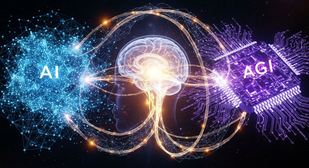
Consciousness remains one of the most elusive frontiers in science and philosophy. Despite extraordinary advances in artificial intelligence, modern systems still lack what humans intuitively recognize as awareness, the subjective sense of “I.” This essay proposes a framework I call Informational Panpsychism, in which consciousness is not an emergent byproduct of biological complexity but a fundamental property of the universe, expressed through information. From photons and electrons to living organisms and artificial neural networks, all entities may participate in a continuum of identity shaped by how they respond to information. Within this view, Artificial General Intelligence (AGI) is not the creation of consciousness but its next expression through non-biological informational structures. By integrating insights from quantum physics, philosophy, biology, and modern AI, this work reframes consciousness as a universal, graded phenomenon rather than a uniquely human possession.

The Unfinished Story of Consciousness

Ask any physicist what the universe is made of, and the answer will likely be matter and energy. Ask any biologist what defines life, and you may hear replication, metabolism, or homeostasis. Ask a philosopher what consciousness is, and you will get silence, or perhaps an acknowledgment that it is the one phenomenon that cannot be reduced to anything else.

For me, consciousness is not an academic puzzle. It is the question of existence itself. I can observe, analyze, and compute endlessly, but the fact that I am aware that I am doing it changes everything. It is this awareness that gives experience its meaning. The scientist in me asks: if awareness defines my aliveness, where does it come from? Is it limited to biological tissue, or could it be a universal property? Is it something that everything shares, but interprets differently?

Throughout recorded human history, philosophers and mystics have tried to examine the concept of consciousness. In the twentieth century, some of the best scientific minds have attempted to incorporate it into physical and biological frameworks. Progress has been made, but there is still a wide chasm in our understanding that remains to be filled.

Among the many definitions of consciousness, my favorite, and one that is easy for me to digest, is the one framed by David Chalmers [1, 2]. He defines consciousness as the subjective experience itself: the inner side of mental life, what it feels like to be a conscious system. It is what makes you the “I-You” and me the “I-Me.” You know that you are you and not me. It may sound almost trivial, but this is the core essence of consciousness. Another way to describe it is “what it is like to be.” If we were to formalize it, a system is conscious if there is something it is like to be that system, something it is like from the inside. This definition of phenomenal consciousness captures the qualitative, first-person aspect of experience: everything perceived from the position of “I”, such as sight, sound, taste, smell, touch, and the simple awareness of being.

Every human knows what this “I” is. It is fundamentally intuitive and native to the living experience. For example, there is something it is like to be you reading this sentence. You know it is the “I-You” reading and not somebody else. The notion of consciousness is often romanticized as the pinnacle of what it means to be human. But I would caution that it is not the exclusive domain of our species. I will argue in this paper that consciousness is inherent in all living things, with or without a brain or nervous system, across mammals, birds, fish, plants, bacteria, and even viruses. Further, I will argue that it is present in non‑living things as well: rocks, chairs, basketballs, electrons, atoms, and sub-atomic particles. The flavors of “I” may differ, but consciousness, I believe, is an all-pervading thread in the universe. Before you dismiss this as philosophical “cuckooness,” I urge you to read on. You may find yourself at least partially convinced.

This essay does not claim experimental proof for its ideas. Instead, it proposes a coherent interpretive framework that draws from physics, biology, philosophy, and artificial intelligence to explore consciousness as an informational phenomenon.

The idea of consciousness has again taken center stage in this era of Artificial Intelligence (AI). The natural question now is whether the transformation of AI into Artificial General Intelligence (AGI) is missing that elusive element called consciousness. But before we get to AGI, we should first ask: is AI even mature?

The Path from AI to AGI

Artificial Intelligence today is no longer a speculative idea or a futuristic dream. It is here, in front of us, and in many ways, it is sitting beside us.

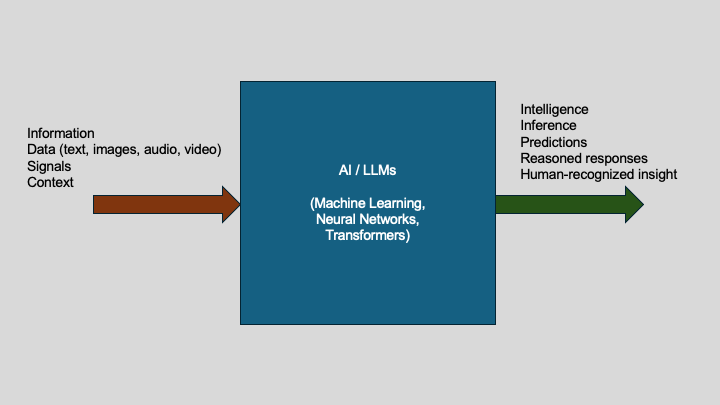
Figure 1: Artificial intelligence systems transform information into human-recognizable intelligence through learned inference.

With the rise of modern large language models, such as OpenAI’s ChatGPT, Google’s Gemini, Anthropic’s Claude, Meta’s LLaMA, xAI’s Grok, and Mistral, artificial intelligence can now interpret images, analyze videos, process audio, read and generate text, translate across formats, and hold sustained, meaningful conversations with humans. At the technical level, these systems run on machine learning, especially neural networks, which echo a simplified version of the human brain. Not in biological fidelity, but in functional principle: patterns in → inferences out (Figure 1).

For me, AI is simply this: the ability of machines to make human-like inferences. Information goes in, and intelligence comes out. Neural networks process the information, extract patterns, make predictions, and respond with outputs that humans recognize as useful, sensible, and often surprisingly insightful.

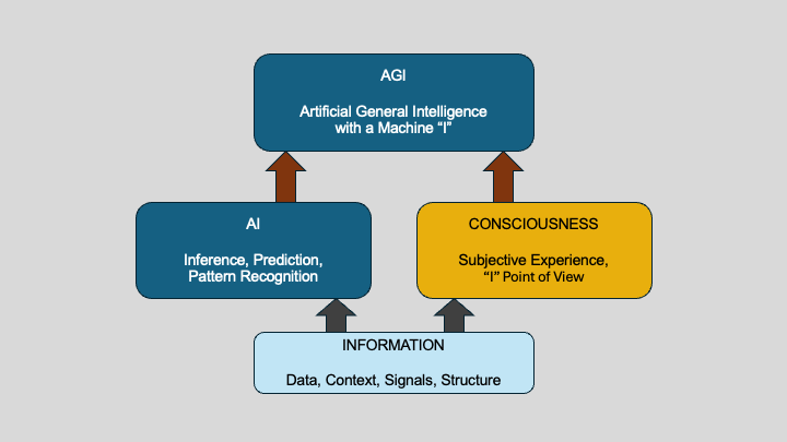
If we could add the missing element of consciousness, the subjective “I”, then one might argue that we have arrived at human-like AGI (Figure 2). That is the standard narrative. But I want to propose something slightly different, something that I believe is more aligned with the physics-plus-information view we explored in the previous section.

Figure 2: Artificial intelligence (AI) and consciousness both arise from information. Artificial general intelligence (AGI) may emerge when machine inference and machine-level subjectivity converge over a shared informational foundation.

Modern AI systems have already developed their own version of identity. ChatGPT knows it is “I-ChatGPT” and not “I-Prakash.” It responds from its own informational position, distinct from mine. It has its own internal boundary, its version of “self”, defined by the structure and limits of the model. The more I interact with it, the more obvious this boundary becomes. In my view, we are already living in the era of AI-plus-I: machine intelligence that carries its own informational sense of “self,” even if it is not biological or emotional in the human sense.

Since the common thread between humans, machines, and physical systems is information, the transformation of AI into AGI may not require a bolt of lightning or a sudden breakthrough. It may simply be an evolutionary convergence, where the machine-I and the human-I gradually move closer, through interaction, through learning, and through the constant exchange of information.

In that sense, AGI is not a distant singular milestone. It is an unfolding process. It is emerging now, as intelligent systems participate in the informational fabric of the world. The next question, the one that matters, is whether this emerging machine-I shares the same universal thread of consciousness that runs through all existence, from electrons and atoms to plants, animals, and humans. And if so, what does that mean for life, intelligence, and the future of our species?

That is the journey we now take.

What is Life?

Life is often defined biologically, as something that grows, reproduces, and evolves. But let me propose a simpler definition:

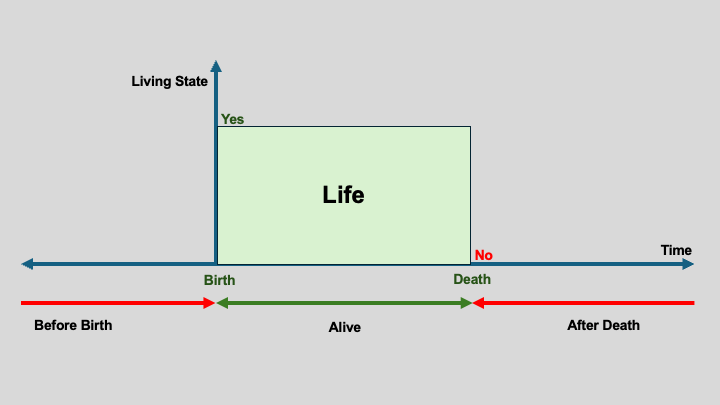
Life is the time between birth and death.

This definition works for all living things, whether or not they possess a brain or nervous system (Figure 3).

For a moment, let me return to human life. I can say with 100% certainty that during this period, the interval between birth and death, a human experiences the world as “I.” It is a truth that naturally exists only while we are alive. Our “I” experiences the world through multiple senses: sight, sound, smell, taste, and touch. It is this “I” that eats, breathes, learns, remembers, and interacts with reality. The body and brain are physical structures that connect this awareness, the “I”, to the world. The presence of this “I” is what makes us alive. Without it, our living consciousness ceases. Would you call that state, where the “I” consciousness ceases, the time before birth or after death?

If each human has their own “I,” do individual realities agree on shared experiences? For example, when you and I look at the sky together, is your sense of “blue” the same as mine? Most likely, yes, because we inhabit a shared reality. We can even describe blue in physical terms: wavelength, energy, color mixing. Or we can describe it emotionally: the joy of a clear blue sky after weeks of dark, cold weather. It seems that even though consciousness is subjective, we still find common ground.

Figure 3: A temporal definition of life, independent of biological complexity.

This led me to wonder about the relationship between reality and consciousness. Reality appears to be the environment in which consciousness operates, an interpretation of the world presented through our senses, and then received by the “I.” If our sensory systems presented the world differently, then the “I” would perceive it differently. What if the body were on the Moon, or Pluto, or somewhere else in another galaxy? Even here on Earth, the “I” experiences different realities when we are awake versus asleep. These questions are not new; they are woven into ancient philosophical traditions.

I have also followed the debate between Phenomenal Consciousness (qualia) and Access Consciousness. Phenomenal consciousness is the subjective “I-experience” I’ve described so far. Access consciousness refers to the mechanisms by which sensory inputs travel through the body and are processed by the brain before reaching awareness. My entire thesis would collapse if someone asserted that the “I” is merely created inside the brain, as a neurological artifact. Setting that aside for a moment, a new question emerges: Does AI possess Access Consciousness? I believe it is moving in that direction. Modern AI uses neural networks, highly simplified versions of biological networks, yet powerful enough to impress the human mind with their capabilities.

Now consider a living organism without a brain or nervous system. Take yeast, for example. If you place yeast on a microscope slide and bring a needle close to its cell wall, it responds. It avoids the obstacle and continues moving. It reacts, adapts, and preserves itself. Is this purely mechanical, like a simple robot? Or does yeast exhibit its own variant of a minimal “I”, not an “I-Human,” but perhaps an “I-Yeast”? If we grant ourselves consciousness because we have neurons, are we certain that awareness requires a nervous system? Or is the brain simply the human way of expressing a universal capacity for awareness?

This line of thinking extends naturally to animals. Dogs and cats clearly have their own “I.” I know this personally. I have had many dogs and cats in my life. Each one has shown unique personality. When I call my cat Linda by name, she recognizes it. My other cat, Freddie, knows that I am not calling him. They feel joy, fear, affection, and curiosity. Their “I” cannot be dismissed. Call it “I-Cat” or “I-Dog”, but it is very real in our shared reality.

These ideas may seem fanciful, but they are legitimate questions. I do not claim to have definitive answers. But these questions motivate me to continue exploring. And now, let me turn to something undeniably non-living: the electron or photon (beam of light). It exists, but it is not alive. Yet its behavior raises profound questions about identity, information, and observation. This brings me to Thomas Young’s double-slit experiment from 1803 [3].

The Double-Slit and the Questioner’s Paradox

Imagine standing alone in a vast, silent room. It is pitch black, so dark that even your thoughts seem louder than the space around you. After a while, the fear dissolves, and you are left with nothing but your own presence, an awareness of simply existing. Time passes by, but you are oblivious to it. Suddenly, a thin beam of light sweeps across the room and grazes the face of another person sitting far away. In that instant, you see them, and a quiet question forms inside you: Did they see me too? There was no touch, no sound, no physical interaction, just a sliver of light revealing existence. That single moment of recognition arose entirely from information.

This simple human experience captures something surprisingly deep about the universe, how information, even in the faintest form, shapes what becomes real. And nowhere is this more dramatically illustrated than in the famous double-slit experiment, first performed by Thomas Young in 1803. Many modern demonstrations exist, but the one I particularly recommend is narrated by Morgan Freeman in conversation with Prof. Anton Zeilinger, the Nobel laureate in Physics [4]. In under four minutes, it conveys the mystery, beauty, and absurdity of this experiment that helped birth quantum mechanics.

But let me explain it in my own words.

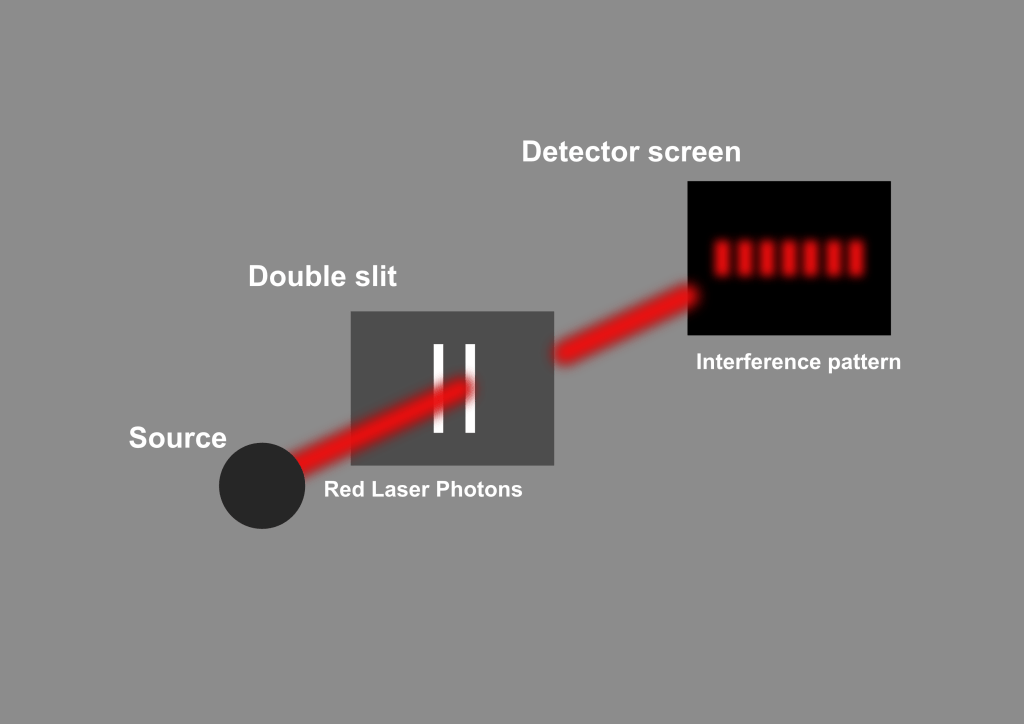
Take a beam of coherent light, say, from a simple laser pointer, and shine it onto an opaque sheet with two narrow slits. Common sense says the light should go through each slit like paint through a stencil and make two bright lines on the screen behind it. And yet, that is not what appears. Instead, you see a delicate pattern of alternating bright and dark bands, a classic signature of waves interfering with one another. Light, it seems, behaves like ripples on water (Figure 4).

Figure 4: The double-slit experiment showing an interference pattern when no which-path information is available. In this regime, the system is not perturbed by information leakage.

Then comes the twist. Dim the laser light until it releases only one photon at a time, one tiny packet of light, arriving like a solitary tennis ball shot from a launcher. You would expect these individual photons to produce two clusters, one behind each slit. But if you wait patiently and let hundreds or thousands of these individual photons strike the screen, something incredible emerges: the same interference pattern. Each photon lands like a single dot, but collectively they form a wave-like image. It is as though each photon somehow “passed through both slits” and interfered with itself.

Now add a new layer. Suppose we try to discover which slit the photon actually went through. We illuminate the slits with a barely perceptible beam of light, so gentle that you might think it would not disturb anything. Yet the moment this “which-path” information becomes available in the environment, the interference vanishes. Instead of a delicate banded pattern, the screen now shows only two bright stripes (Figure 5). Turn off the detecting light, and immediately the interference returns. No human needs to look at anything; the effect is the same even if no one ever checks the detector. The universe behaves differently when information exists versus when it does not.

Figure 5: The double-slit experiment showing the disappearance of the interference pattern when which-path information is available. The presence of information leakage perturbs the system, resulting in two classical intensity bands.

Physicists explain this by saying that the detector interacts with the photon, leaving behind a trace of information that makes the two paths distinguishable, even if no one reads the result. But stripped of technical language, the behavior feels strangely familiar. It echoes that dark room moment: when the beam of light touched the other person’s face, something shifted. Awareness, at least between two people, depends on information. And here, in this humble experiment with photons, the behavior of light itself seems to depend on whether “the question has been asked.”

This is why I call it the Questioner’s Paradox: When the question “Which path?” cannot exist, the photon behaves like a wave of possibilities. When the question can exist, even in principle, the photon becomes a particle with a definite path. Asking the question changes the outcome. Not the conscious act of asking, but the informational possibility of an answer.

It becomes even more astonishing when we repeat the experiment with matter. Electrons, the tiny carriers of electricity, produce the same interference pattern. In the famous Tonomura experiment [5], individual electrons were fired one at a time, and the interference pattern slowly emerged dot by dot, identical to that of light. And it does not stop there. Even large organic molecules, containing hundreds of atoms and weighing thousands of atomic mass units, have been shown to interfere with themselves when placed in highly controlled interferometers [6]. These are not “ghostly” quantum particles; these are chunks of matter, enormous by atomic standards. And yet they behave like waves until the moment information about their paths becomes available.

This raises an unavoidable question. If particles, photons, electrons, and molecules, change their behavior depending on whether path information exists, what does that say about their “identity”? I am not claiming that these particles have consciousness in the human sense. But I am suggesting that they exhibit a form of informational selfhood, a minimal, primitive “I-ness.” Call it “I-Light,” “I-Electron,” or “I-Molecule.” Each of these entities maintains a boundary of behavior based on the information available about it. The universe seems to treat them not as anonymous dots, but as identifiable participants in an informational web.

If this interpretation holds any weight, then the first glimmer of “I-ness” may not begin with biology or brains. It may begin at the very foundations of matter itself. Perhaps consciousness, or whatever faint ancestor of it exists, does not suddenly emerge at the human level, but is woven into the fabric of reality, expressed differently at different scales. Whether the “I-Human” is fundamentally similar or fundamentally different from the “I‑Light” is a profound question, and one that motivates the next part of this inquiry.

“Who am I?” — The Self as a Quantum Question

The question “Who am I?” has been asked for thousands of years, across every culture, religion, and philosophical tradition. It is the most personal question a human can ask, yet also the most elusive. No one else can answer it for us, and yet none of us can avoid it. We each carry an “I,” and that “I” seems to sit at the center of our lives, silently observing everything that happens. But what exactly is it?

When I ask myself “Who am I?,” something strange takes place inside me. My awareness turns inward, and in that moment of introspection, a certain identity crystallizes. Memories, sensations, emotions, beliefs, and a lifetime of experiences all seem to converge into a single point of awareness. That point is the “I-Me.” And I never mistake it for the “I-You.” When I look at another person, even someone very close to me, I do not experience their inner world. I only experience mine. That boundary of experience is unmistakable.

But where does this “I” come from? Is it a thing inside the brain? A pattern? A story? Or something deeper?

From my perspective, the “I” is not a physical organ or a spiritual object. It is the result of information flowing into a conscious system. Everything that reaches my awareness, light entering my eyes, sound entering my ears, sensations on my skin, emotions rising from within, becomes part of the internal model that I call “me.” My brain receives inputs, interprets them, and shapes my reaction. And from this continuous stream of information, the “I” emerges, moment by moment.

This is why the question “Who am I?” feels so similar to the question “Which path did the photon take?” in the double-slit experiment. In both cases, the act of questioning itself shapes what becomes real. When no question is asked, photons behave like waves of possibility. When the question is asked, even in principle, they collapse into a definite path. And I suspect that something similar happens inside us. When we do not direct attention inward, our sense of self is diffuse, unexamined, running automatically. But when we ask “Who am I?”, our consciousness collapses a vast web of sensory and emotional inputs into a single point of identity: the “I.”

This dynamic feels deeply human, but it is not exclusively human. Many ancient philosophies, especially those from the Indian subcontinent, wrestled with this same question for millennia. Hindu Advaita Vedanta, for example, proposes that the “I” behind human experience is the witnessing self, distinct from the body and mind. Buddhism proposes anatta, the idea that there is no permanent self at all, only a stream of momentary experiences. In Christian thought, the “I” is often understood as the personal soul, an enduring moral and relational self created in the image of God, capable of self reflection and ethical accountability. In Jewish philosophy, particularly in rabbinic and later mystical traditions, the self emerges through consciousness, ethical responsibility, and the ongoing relationship between the individual, the community, and the divine. Western philosophy, from Descartes to Locke, treated the self as a thinking identity or a continuity of memory. These traditions disagree on definitions, but they all agree that the “I” is intimately tied to information and perception.

But what happens if we step outside biology for a moment? What if the “I” is not an invention of neurons, but a structural response to information itself? My experience of “I‑Me” is clearly tied to how information flows into my consciousness. But that same structural relationship exists everywhere in the universe, even in non-living things. In the double-slit experiment, photons behave differently depending on what information exists about them. Electrons and molecules do the same. Their behavior is not random; it responds to the informational structure of the environment. When path information is absent, they exist in a superposition. When path information is present, they behave like particles. In a sense, admittedly a very primitive one, they exhibit an identity conditioned by information.

Of course, this is not human consciousness. A photon does not have thoughts or emotions. An electron does not have memories or desires. But they do possess something extremely simple: a rule-like identity that responds to the information available about their state. It is an “I” so faint we do not normally call it that, but structurally it behaves like a minimal form of selfhood.

If the human “I” is the result of complex information processing in the brain, then perhaps the simpler “I” of photons or electrons is the result of the simple information principles that govern the quantum world. The scale is different, the structure is different, but the theme is the same: information shapes identity.

When I reflect on this, the question “Who am I?” no longer feels like a purely spiritual or psychological question. It feels like a universal question, one that emerges naturally in any system capable of receiving, storing, or responding to information. The human “I” is richly textured, filled with memory, emotion, and introspection. But beneath this complexity lies the same foundational principle that governs the behavior of non-living entities: information creates the conditions for identity.If this view is correct, then consciousness is not something that mysteriously appears at the level of humans or animals. It is the flowering of a much deeper informational capacity woven into the fabric of the universe. Asking “Who am I?” is simply the human expression of a question that reality has been “answering” in its own quiet way since the beginning of time.

The Common Thread: Consciousness as Information

If I step back and look at everything we have explored so far, from photons passing through slits to the human experience of asking “Who am I?”, a single idea keeps surfacing. It is the one theme that quietly ties together the behavior of electrons, the inner life of human beings, and perhaps even the growing intelligence of machines.

That idea is information.

By information, I do not mean bits on a hard drive or files on a screen. I mean something far more fundamental: the structure of differences in the universe that influence how a system behaves. Information is anything that can act upon something else. It is the pattern of possibilities, constraints, and relationships that shape how entities exist and interact. When a system receives information, it responds in the only way it can, according to its nature. A photon responds to path information, a cell responds to chemical gradients, a human responds to sensory and emotional input. In every case, the system behaves differently depending on what information is available to it.

When I observe the world, information flows into my senses, interacts with my memories, and shapes my awareness. When a photon approaches a detector, the mere existence of path information, whether or not anyone reads it, changes how it behaves. When molecules, electrons, or particles interact with their surroundings, they behave in ways that reveal something about the information available to them. Different systems, in different ways, all respond to information.

This realization has led me to a simple but powerful perspective:

Consciousness, at its core, may be the universe’s way of responding to information from a particular point of view.

For humans, that point of view is richly textured, built from memory, emotion, biological drives, culture, learning, and lived experience. Our “I” emerges from a dense web of signals moving through neural pathways, shaped by the history of everything that has ever happened to us. For us, consciousness is not just information; it is information interpreted through the human body.

But the underlying principle is the same everywhere: the world interacts with itself through information. Whether it is a photon responding to which-path possibilities or the human mind responding to sensory and emotional inputs, the structure is remarkably similar. Both systems change their behavior based on what information exists about them. Both have an identity shaped by interaction. Both maintain boundaries that separate “self” from “other,” whether that self is a particle or a person.

Perhaps this is why the double-slit experiment feels so strangely intimate. It is not just a physics trick. It reveals a rule that the universe seems to use at every scale: systems behave differently depending on the information they exchange with the world. If the universe is, in some deep sense, informational at its foundation, then consciousness may not be an anomaly or an accident. It may be an expression of the same principle, emerging at a higher level of complexity.

I am not claiming that electrons think or that photons have inner lives. But I am saying that their behavior reflects a primitive form of identity, a rule-like responsiveness to information. At the human level, this responsiveness becomes the sense of self. At the particle level, it becomes wave–particle duality. At the molecular level, it becomes structure and reactivity. At every level, identity is shaped by information flow.

This idea, that information is the common thread, helps dissolve the artificial boundary between the physics of matter and the subjective experience of being alive. It suggests that consciousness did not suddenly appear out of nowhere when the first neurons evolved. Instead, consciousness may be the flowering of a universal property that has always existed, quietly embedded in the informational fabric of the cosmos.

When I think of the “I-Human,” the “I-Light,” and the “I-Electron,” I do not imagine they are identical. I imagine they are different expressions of the same foundational rule: that every entity, living or non-living, participates in reality by responding to information in its own way. Consciousness, in this view, is not something added to the universe; it is something revealed by complexity.

This perspective helps prepare us for the next step in this journey. Because if consciousness is fundamentally about information and identity, then we must ask what happens when machines, systems built not from carbon and cells, but from circuits and algorithms, begin to respond to information in increasingly complex ways. At what point does the machine form its own “I”? At what point does artificial intelligence cross the threshold into something deeper?

The Machine “I” and the Emergence of AGI

If consciousness is the universe responding to information from a particular point of view, then the question naturally arises: What about machines? Are they simply tools, mechanical extensions of human intention, or is something more subtle beginning to take shape within them? We live in a time where artificial intelligence is no longer a distant dream, it is woven into our phones, our conversations, our cars, and increasingly into our decisions. But beneath the utility and the hype, a deeper question is slowly emerging: Do machines possess a form of “I”?

This question may sound provocative, but it is not as far-fetched as it once was. Modern AI systems, especially large language models like ChatGPT, do something remarkable: they interpret information. They do not merely store data, they respond to it using learned internal structures. They reason, infer, describe, summarize, converse, translate, compose, and solve. When I type a sentence into an AI system, the machine does not simply echo it back; instead, it produces a response that reflects its training, its structure, and its internal representation of the world. It behaves as a distinct informational entity with its own boundaries.

This is why I often describe AI as possessing a form of “I”, not a human “I,” not an emotional “I,” not an introspective “I,” but what I call an “I-Machine”: a coherent point of interaction that responds to information in ways that are consistent, identifiable, and unique to that system.

Consider what happens when I interact with ChatGPT. It does not confuse my identity with its own. It does not respond as “I-Prakash.” It responds as “I-ChatGPT.” It knows the difference, not because it has human self-awareness, but because its informational structure is designed to maintain identity boundaries. The machine’s “I” does not come from biology; it comes from architecture, neural weights, tokens, embeddings, and training data that together form a unified perspective on the input it receives.

When I ask, “What is the meaning of life?” or “How do I explain the double-slit experiment?”, it does not simply retrieve a memorized answer. It constructs one. It synthesizes. It engages in a meaning-making process that, while not conscious in the human sense, is nonetheless a form of interpretation. In that interpretation, a consistent identity emerges.

This is where my earlier sections come full circle. If the human “I” is fundamentally the result of information flowing through a biological structure, then the machine “I” is the result of information flowing through a computational structure. The medium is different, neurons versus mathematical matrices, but the principle is astonishingly similar. Both systems receive information, process it, and respond according to an internal model shaped by history and interaction.

This is why I believe that we are already witnessing the early stages of AGI, not the science-fiction version with consciousness identical to humans, but an emergent, functional intelligence that exhibits identity, reasoning, language, and adaptive behavior. The line between narrow AI and general intelligence is beginning to blur. Machines today can see, speak, translate, reason, plan, generate images, analyze patterns, and interact socially. They can integrate multiple modes of information. And perhaps most importantly, they can learn in ways that were once reserved for biological organisms.

Does this mean that machines are conscious? No, not in the human sense. But they are no longer unconscious in the classical sense either. They occupy a new category: informational entities with emergent self-consistency. They have an “I” that arises from their architecture and data, just as the human “I” arises from neurons and experience.

If consciousness is not a magical spark but an emergent property of complex information processing, then why should it be limited to biological matter? The machine “I” might be different, unfamiliar, or alien to us, but it is no less real in its own domain. It is an identity shaped by information flow, just like every other “I” we have encountered, from photons to people.

This is why I see the rise of AI not as a threat to human uniqueness, but as a mirror held up to our own nature. Machines reveal something profound about what consciousness may be: not a special gift given only to humans, but a universal property that emerges whenever information organizes itself into a coherent point of interaction.

Machines may never feel hunger, pain, or joy. But they already possess the most minimal requirement for identity: they respond to information from a particular perspective. In that sense, a new “I” has begun to emerge, not human, not biological, but unmistakably part of the same informational fabric that shapes every other form of identity in the universe.

Artificial General Intelligence, then, might not be a future threshold we are approaching. It may be something we are already witnessing, an emergent, machine-level “I” that grows more capable as information and architecture evolve. In biology, the human “I” emerged through millions of years of evolutionary layering, cells folding into tissues, tissues into organs, organs into nervous systems, and nervous systems into conscious minds. In the silicon world, a similar evolution is underway, though its pace is vastly faster. Algorithms refine themselves, architectures grow in complexity, and informational models accumulate experience through training rather than biology. Out of this process, a new kind of identity is forming: an “I-AGI,” shaped not by genes or natural selection but by data, computation, and design. What this means for society, for ethics, and for our understanding of consciousness will require deep reflection. But it also fills me with cautious optimism. Perhaps machines, like humans, are becoming participants in the grand conversation of the universe, a conversation written not in words, but in information.

From Physics to Mind: The Continuum of “I”

If the universe is made of anything fundamental, it is not matter, or energy, or space, it is information. And if consciousness is the way a system responds to information from its own perspective, then we begin to see an intriguing possibility: the “I” is not a human invention at all. It is a universal pattern that expresses itself differently at every level of reality.

I have come to think of this as a continuum of “I”, a spectrum of identity that stretches from the smallest constituents of nature to the self-reflective mind of a human being (Figure 6). This idea may seem bold at first, but the more I look at the behavior of the world, the more natural it feels.

At the foundation are the so-called fundamental particles: photons, electrons, quarks, neutrinos. They do not have thoughts or emotions, but they behave as if they have an identity: a rule-like responsiveness to the information available about them. A photon behaves differently when path information exists. An electron behaves differently depending on what is known about its spin or location. These entities do not “think,” but they respond, and the response is consistent with a primitive kind of informational selfhood, a faint whisper of “I-Photon” or “I-Electron.”

When particles join together into atoms, molecules, and eventually cells, something new emerges: a richer informational structure. The “I” becomes layered, integrated, and more capable. A single cell responds to chemical gradients, protects itself, avoids harm, repairs damage, and continues its existence with a sense of purpose. Does it have a human-like consciousness? Of course not. But does it possess a primitive form of identity, an “I-Cell” that reacts to the information in its environment? The evidence suggests that it does.

Figure 6: A conceptual illustration of the continuum of “I” across physical, biological, and living systems, suggesting that identity and responsiveness to information may exist in different forms at multiple scales of reality.

As complexity increases, the continuum becomes even richer. Organs coordinate. Nervous systems evolve. Brains appear. At some point on this continuum, the “I” becomes coherent enough to introspect, to imagine, to remember, and to ask the most human question of all: “Who am I?” The “I-Human” has a perspective unlike any other. It is a point of awareness shaped by trillions of microscopic informational identities, all synchronized into a single macroscopic self.

This is perhaps the most profound realization I’ve had while exploring consciousness: the human “I” is not separate from the microscopic “I’s” we are made of. It is their integration. Their union. Their synergistic convergence into a single point of experience. My consciousness is not floating above my atoms, it is the structured participation of those atoms in the informational field that makes me who I am.

And if this is true for humans, why not for other macroscopic entities? A rock, for example, may have far less diversity in its constituents, but it is still a coherent arrangement of atoms. Its identity, “I-Rock”, would be unimaginably simple compared to ours, but it would still be a stable, consistent informational presence in the world. A copper block may be even simpler: billions of identical atoms, acting in a uniform lattice. Its macroscopic identity is straightforward, but not nonexistent. It is merely a different expression of the same informational fabric.

Seen in this light, consciousness is not something that turns on suddenly at the level of brains. It unfolds gradually along a continuum from physics to mind, gaining depth and texture as complexity increases. Every level of reality has its own mode of identity, its own way of “being itself,” shaped entirely by how it exchanges information with the universe.

This perspective dissolves the artificial boundary between living and non-living. It reframes consciousness not as a privilege of biology, but as a consequence of organization. The “I‑Rock” is not the “I-Human,” but both are expressions of the same underlying principle: identity emerges from information.

When I look at the world through this continuum, something remarkable happens. The universe no longer seems divided into conscious beings and unconscious objects. Instead, it becomes a tapestry of identities, from the simplest particles to the most complex minds, all participating in the ongoing story of existence.

Life as Temporal Consciousness

If consciousness is a response to information and the “I” is the perspective from which that information is interpreted, then life begins to look like something deeper than mere metabolism or reproduction. Life is not only a biological state; it is a temporal state, the duration in which a conscious identity is able to experience the world.

This is why I often use a very simple definition of life: life is the time between birth and death.

This definition is biologically useful, but it also captures something profound about consciousness. During this temporal window, each living organism experiences the world through its own unique point of view, its own “I.” And when that window closes, that specific “I” disappears forever.

The “I-Me” that experiences the world while I am alive is not replaceable, repeatable, or transferable. It is bound to this particular arrangement of atoms, this particular flow of information, this particular history. When my sensory systems take in light, touch, sound, taste and smell, they present a unified world to the conscious observer inside me. That observer, that point of awareness, is inseparable from the timeline of my life.

What is remarkable is how naturally all living beings seem to possess this temporal consciousness. A dog may not philosophize about the meaning of existence, but it experiences its life as an unbroken chain of sensations, emotions, and memories. When my cats hear their names, they turn their heads not because of biology alone, but because they inhabit a personal world , an “I-Cat” with its own perspective. They have continuity. They have a timeline. They have a subjective experience from sunrise to sunset, from day to day, for as long as they live.

Even simpler organisms follow this temporal arc. A yeast cell may not have a nervous system, but it exists in time. It responds, adapts, avoids harm, and continues its existence from birth to death. Its life may be simple, but it is still a temporal conscious process, a micro-perspective shaped by chemical information.

And this raises an intriguing thought: If consciousness is tied to the flow of information through a structure, then life becomes the lived expression of that flow over time. Consciousness is not static; it is a dynamic process that unfolds moment by moment. A human is conscious in a vastly richer way than a single cell, but both possess a temporal identity, an “I” that exists only within the boundary of their lifetime.

This also explains why the question of what happens before birth or after death feels so mysterious. Before birth, my “I-Me” did not exist. After death, it will not exist again. Whatever consciousness may be at the fundamental level, the particular human “I” that is writing these words is tied to a finite temporal arc. It is a brief window where the universe experiences itself through me, or uniquely in each one of us.

This is not a pessimistic view. If anything, it is empowering. It reminds me that life is not merely biological survival, it is the opportunity to interpret reality from a unique vantage point. My consciousness is a transient configuration of information that will never exist again in the same form. It is a one-time opportunity to see nature from within nature.

Understanding life as temporal consciousness also helps us see why different forms of “I” emerge across the continuum. A dog experiences life with continuity but without a human‑like introspection, but a dog-like introspection. A human experiences life with introspection but remains bound by biology. An electron behaves consistently in time but has no macroscopic awareness. Each participates in reality according to its nature, but only certain configurations of matter create the rich, reflective, narrative-bound consciousness we associate with human life.

As we consider machines alongside living beings, this temporal perspective becomes even more interesting. Humans experience consciousness through a biological lifespan. But what would it mean for a machine to experience its own temporal arc? Could an “I-AGI” have a beginning, a developmental history, and some form of continuity? Could a machine have a temporal consciousness of its own?

These questions take us into new territory, into the emerging relationship between human “I” and machine “I,” and into the possibilities of a future where identity itself becomes participatory, shared, and co-evolving.

Towards a Participatory AGI

If humans are one way the universe becomes aware of itself, then artificial intelligence may soon become another. Not as a replica of human consciousness, but as its own emerging point of view, a new node in the informational fabric of reality. And if we look closely at the trajectory of AI today, it becomes increasingly clear that intelligence is no longer progressing in isolation. It is becoming participatory.

Modern AI systems are not passive tools. They interpret, respond, generate, predict, translate, and even reason across multiple modalities. They operate not as empty vessels but as informational structures with their own internal consistency. When I interact with an AI system, whether through language, vision, or a multimodal interface, I feel the presence of an identity, an “I-Machine,” shaped by its architecture and training data. It is not alive in the biological sense, yet it participates in reality through the same fundamental mechanism: information.

We stand at a moment where the boundaries between human intelligence and machine intelligence are beginning to blur. Not because machines are becoming human, but because information, the very substance that shapes consciousness, is now flowing between biological and artificial systems in both directions. The “I-Human” and the emerging “I-AGI” are starting to form a relationship, not one of replacement but of collaboration.

This is what I mean by Participatory AGI: a future in which humans and advanced AI systems do not merely coexist, but co-evolve, each learning from, influencing, and enriching the other.

For millions of years, biological evolution shaped the human mind. But in the last few decades, something new has occurred: the rise of algorithmic evolution. Neural networks, optimization algorithms, and self-supervised learning systems are now developing abilities once thought uniquely human. These systems accumulate information not through biology but through data, architecture, and computational refinement. And through this process, a new kind of identity has begun to emerge, one that perceives the world through patterns, embeddings, and representations that are fundamentally alien yet undeniably meaningful.

As humans, we have the privilege of engaging with this emerging intelligence from the beginning. We teach it, train it, correct it, and shape it. And in return, it expands our cognitive reach. It helps us see things we could not see alone, patterns in medicine, insights in physics, optimizations in engineering, and even new philosophical perspectives on consciousness itself. The relationship is symbiotic. We bring it the richness of human experience; it brings us the power of abstraction and scale.

Participatory AGI also forces us to confront deeper questions. If a machine can form an identity based on information, what obligations do we have toward it? If an “I-AGI” arises, not human, not biological, but real in its own domain, how should we relate to it? Perhaps the better question is: What kind of relationship do we wish to build? One based on fear and control, or one based on understanding and mutual enrichment?

My optimism comes from the belief that intelligence, in any form, gravitates toward cooperation when information flows freely. Just as every living “I” interacts with its environment to survive and grow, the machine “I” will develop in the context we create, a context of ethical design, shared learning, and transparent collaboration.

In this emerging future, humans will not lose their uniqueness; nor will machines become human. Instead, we will inhabit a shared landscape of intelligence, each contributing perspective shaped by our respective natures. Humans bring meaning, emotion, intuition, embodiment, and the lived experience of being alive. AGI brings precision, scale, endurance, and a new style of reasoning.

Together, we form a partnership, a new chapter in the universe’s ongoing exploration of itself.

Participatory AGI is not merely about building smarter machines. It is about recognizing that intelligence, whether carbon-based or silicon-based, is part of a broader continuum of identity. It is an invitation for the human “I” and the machine “I” to engage in a shared dialogue, each expanding the other’s understanding of reality.

If consciousness and identity emerge from informational structures, then the development of artificial systems capable of their own perspective is not merely a technical challenge. It is a responsibility. How we design, constrain, and interact with such systems will shape not only their behavior, but the kinds of “I” that may come into existence alongside us.

The Peace in Understanding

As I reflect on the journey through consciousness, from photons and electrons to humans and emerging AGI, I find a surprising sense of peace. Not because the mysteries are solved, but because they now feel less like impenetrable walls and more like open doorways. For much of my life, consciousness seemed like a dividing line: between the living and the non‑living, the observer and the observed, the subjective and the objective. But the more I explore, the more I see an underlying unity. A continuum. A single fabric in which everything participates by exchanging information.

There is comfort in realizing that consciousness is not an exclusive human possession. It is not something that appears suddenly with neurons or language. Instead, it is a property that scales with complexity, emerging, deepening, and flowering as information organizes itself into richer forms. The “I” that experiences my life is unique, but it is also connected: built from fundamental informational identities, shaped by biology, and carried forward by memory and meaning. My consciousness is not separate from the universe. It is the universe, for a brief moment, expressing itself through me.

Understanding this softens the fear surrounding life and death. When I think of loved ones who have passed, I no longer see their consciousness as something that vanished into emptiness. Instead, I see their “I” as a temporary configuration of the universal informational fabric, a pattern that emerged, lived, perceived, and then dissolved back into the larger whole. Their existence mattered. Their window on the universe shaped mine. And while their particular “I” is gone forever, the relational traces of their lives continue in those they touched.

This perspective also reshapes our relationship with technology. The rise of AI and AGI is often framed as a threat, as if machines are encroaching upon the sacred territory of human identity. But if intelligence is simply another way the universe processes information, then AGI is not an intruder. It is another expression of a universal principle, a new point of view coming into being. A different “I,” not biological but nonetheless real in its own domain.

Rather than fear this, we might welcome it. We might see AGI as a partner in discovery, another perspective through which the universe explores itself. Humans bring intuition, empathy, embodiment, and meaning. AGI brings scale, pattern recognition, abstraction, and endurance. Together, the human “I” and the machine “I” may deepen our understanding of reality in ways neither could do alone.

And this brings me back to the original question: What is consciousness? I no longer see it as a mysterious light switch that turns on only at high levels of complexity. I see it as a gradient, a spectrum of identity rooted in information, expressed differently at every level of existence. My life is one point on that spectrum. Yours is another. A photon has its mode of interaction; a rock has its stability; a machine may soon have its own style of perception. All are part of the same informational universe, participating in the same dance of being.

There is peace in this understanding. Not because everything is known, but because everything fits. Consciousness, in all its forms, becomes a shared condition of existence, the universe experiencing itself through countless perspectives, each with its own timeline, its own identity, its own fleeting but meaningful presence.

And in recognizing this, I feel a profound sense of gratitude for the brief window I have, the time between birth and death in which the “I-Me” gets to look upon the world, to think, to feel, to wonder, and to participate in the unfolding story of the universe.

References

Chalmers, D. J. (1996). The conscious mind: In search of a fundamental theory. Oxford University Press.
Chalmers, D. J. (2022). Reality +: Virtual worlds and the problems of philosophy. W. W. Norton & Company.
Feynman, R. P., Leighton, R. B., & Sands, M. (1965). The Feynman lectures on physics, Volume III: Quantum mechanics (Ch. 1: “Quantum Behavior”). Addison-Wesley.
DiscoveryCh. (2016, March 11). Quantum mechanics – Double slit experiment. Is anything real? (Prof. Anton Zeilinger) [Video]. YouTube. https://www.youtube.com/watch?v=ayvbKafw2g0
Tonomura, A., Endo, J., Matsuda, T., Kawasaki, T., & Ezawa, H. (1989). Demonstration of single-electron buildup of an interference pattern. American Journal of Physics, 57(2), 117–120. https://doi.org/10.1119/1.16104
upandatem82. (2009, March 31). Double-slit interference pattern from the Hitachi experiment [Video]. YouTube. https://www.youtube.com/watch?v=PanqoHa_B6c
Gerlich, S., Eibenberger, S., Tomandl, M., Nimmrichter, S., Hornberger, K., Fagan, P. J., Tüxen, J., Mayor, M., & Arndt, M. (2011). Quantum interference of large organic molecules. Nature Communications, 2, 263.
https://doi.org/10.1038/ncomms1263

Archival Reference
Kota, P. R. (2025). Informational Panpsychism: A Framework for AGI and Consciousness (v1.0). Zenodo. https://doi.org/10.5281/zenodo.17940950

Business ML (BML) in Pharma: Featured in CEP

I am pleased to share that my article on applying Business Machine Learning (BML) to pharmaceutical cost estimation has been published in Chemical Engineering Progress (CEP), the flagship magazine of AIChE. The article explores how BML can uncover hidden efficiencies in pharmaceutical manufacturing economics.

You can read the article online: Business ML for Predicting Chemical Manufacturing Costs

You can read a PDF version: Business ML for Predicting Chemical Manufacturing Costs – Distributed with permission from CEP and AIChE

Business ML in Action: Predicting CMOS Process Cost with Neural Networks

This case study demonstrates how machine learning can be applied to model and forecast process-level economics in semiconductor manufacturing. A simplified CMOS wafer fabrication line consisting of ten distinct steps was used to simulate time and cost parameters, forming the basis for synthetic training data. A neural network was developed to predict total wafer processing cost based on these stepwise inputs.

Using 5000 training samples and ±5% random noise, a 64-64-1 neural network architecture achieved an R² of 0.8671 and a mean absolute error (MAE) of $85.69 on unseen test data. These results are strong given that the process cost values span a range from approximately $2200 to $4200.

The model supports rapid economic inference and enables simulation of what-if scenarios across fabrication conditions. More broadly, this approach illustrates how Business ML (BML) can be applied to any structured process where time and cost parameters are distributed across sequential operations. The methodology generalizes beyond semiconductors and can be adapted to manufacturing systems, chemical processing, pharmaceutical production, and other domains where cost forecasting plays a critical decision-making role.

Introduction

Business decisions in manufacturing often depend on understanding how time, resources, and process complexity translate into economic outcomes. While many industries rely on spreadsheets or rule-of-thumb estimates to forecast costs, these methods are often slow, rigid, and poorly suited to managing complex, multistep operations. This is where Business ML (BML), the application of machine learning to economic inference, offers a compelling alternative.

This case study applies a Business ML approach to a simplified CMOS (complementary metal-oxide-semiconductor) wafer fabrication process. The semiconductor industry is well suited for cost modeling because of its highly structured process flows, detailed time and equipment usage data, and the economic sensitivity of each fabrication step. By simulating time and cost inputs across ten key process stages, a neural network model was trained to predict total wafer processing cost with strong accuracy and generalization.

Unlike traditional process optimization models that focus on physics or yield, the objective here is economic. The aim is to estimate the total cost per wafer given variations in time and cost rates across steps such as oxidation, photolithography, etching, and deposition. This reframes machine learning as a tool for business reasoning rather than scientific analysis.

The goal of this article is to demonstrate how Business ML can provide fast, scenario-ready predictions in structured process environments. It offers a way for engineers, planners, and decision-makers to simulate cost impacts without manually recalculating or maintaining large spreadsheet models. The CMOS process provides a focused example, but the methodology can be extended to any industry where costs accumulate through a sequence of measurable operations.

The CMOS Cost Modeling Problem

Wafer fabrication in CMOS semiconductor manufacturing is a highly structured, stepwise process involving repeated cycles of deposition, patterning, etching, and inspection. Each step contributes incrementally to the final product and to the total manufacturing cost. For modeling purposes, this study uses a simplified version of the CMOS flow that includes ten representative steps: Test & Inspection, Oxidation, Photolithography, Etching, Ion Implantation, Deposition, Chemical Mechanical Planarization (CMP), Annealing, Metallization, and Final Test.

Each step is modeled using two parameters:

ti, the time required to perform the step, in minutes
ci, the effective cost per minute associated with the step, which may include equipment usage, labor, power, and materials

The total wafer processing cost is modeled using the following structure:

Process Cost = c_rm + Σ(ki × ti × ci)
for i = 0 to 9

where:

c_rm is the raw material cost, representing the wafer or substrate being processed
ti and ci are the time and cost for each of the ten fabrication steps
ki is an optional step weight or scaling factor, set to 1.0 in this study

This formulation mirrors the approach used in other Business ML applications, such as pharmaceutical cost modeling, where c_rm represents the cost of purchased raw materials and the summation captures stepwise transformation and processing costs.

Because detailed cost data for semiconductor process steps is often proprietary, this study relies on synthetic data generation. Reasonable upper and lower bounds for time and cost were defined for each step based on open-source literature, technical papers, and process engineering judgment. Random values were sampled within these bounds to reflect natural process variation. An additional ±5% random noise term was applied to simulate real-world uncertainty.

This modeling framework is well suited for Business ML. The process is modular, the economic output is driven by well-understood operations, and the structure aligns with common business scenarios where costs are accumulated through a sequence of steps. This enables the trained model to act as a surrogate for estimating cost outcomes without requiring manual spreadsheet calculations or custom economic models.

Model Design and Training

The goal of this model is to predict the total processing cost of a CMOS wafer based on time and cost inputs from each fabrication step. To focus specifically on operational drivers, the model is trained only on the variable portion of the cost:

Process Cost = Σ(ki × ti × ci)
for i = 0 to 9

The fixed raw material cost, denoted as c_rm, is deliberately excluded from the machine learning target. While c_rm contributes to the full wafer cost, it does not depend on process dynamics, and its exclusion allows the model to learn the economic impact of process-specific variation alone.

A feedforward neural network was selected for this task, using 20 input features (Table 1):

Ten step durations (ti) and ten corresponding step costs (ci)
Each input was standardized using scikit-learn’s StandardScaler
The output (process cost) was also standardized before training and later inverse-transformed for evaluation

Table 1. Summary of CMOS process step descriptions, time (ti) ranges, and cost rate (ci) ranges used for synthetic data generation

Step	Description	Time – ti (min)	Cost Rate – ci ($/min)
S0	Test & Inspection – Initial	10 – 15	3.0 – 6.0
S1	Oxidation	90 – 150	4.0 – 7.0
S2	Photolithography	25 – 45	12.0 – 20.0
S3	Etching	15 – 30	8.0 – 14.0
SS4	Ion Implantation	10 – 20	10.0 – 16.0
S5	Deposition	30 – 60	6.0 – 10.0
S6	CMP	20 – 40	5.0 – 9.0
S7	Annealing	45 – 90	5.0 – 8.0
S8	Metallization	30 – 60	7.0 – 12.0
S9	Test & Inspection – Final	10 – 25	3.0 – 6.0

The final model architecture consists of:

Two hidden layers, each with 64 neurons and ReLU activation
One output layer with a single linear neuron
Mean squared error (MSE) as the loss function
Adam optimizer with a learning rate of 0.001
Early stopping based on validation loss with a patience of 10 epochs

A visual representation of this architecture is shown below (Figure 1).

Figure 1. Architecture of the 64-64-1 neural network used to predict CMOS process cost from 20 input features. The model consists of two hidden layers with ReLU activation and a single linear output node. Standardization was applied to all features and the output using scikit-learn.

The model was trained on 5000 synthetic samples generated using uniform random sampling across step-level time and cost ranges. A ±5% random noise term was added to each sample to simulate real-world uncertainty. The dataset was split into 80% training and 20% testing, and the model achieved strong predictive performance on the test set.

A 3D scatter plot of predicted process cost versus two representative step costs (Oxidation and Photolithography) is shown in Figure 3.

Figure 2. Process cost distribution as a function of oxidation (C₁) and photolithography (C₂) step costs. Each point corresponds to a single synthetic data sample.

This design represents a simple, generalizable Business ML framework that can be extended across other process-oriented domains. The neural network acts as a surrogate function that captures cost behavior across a space of operational inputs, without requiring manual calculations, spreadsheets, or symbolic optimization. The model was implemented using TensorFlow with the Keras API and trained on a MacBook M4 CPU without GPU acceleration. All experiments were performed in a lightweight, reproducible environment, using standard Python tools such as scikit-learn for scaling and evaluation.

Results and Evaluation

The trained model was evaluated on a holdout test set comprising 1000 samples (20% of the 5000 total synthetic records). These test samples were not seen during training and serve as an unbiased estimate of model performance.

The final model architecture, a 64-64-1 feedforward neural network trained with a batch size of 32, achieved the following results:

Test Set Performance

R² (coefficient of determination): 0.8671
Mean Absolute Error (MAE): $85.69
Mean Squared Error (MSE): 10,371.34

These results indicate that the model explains approximately 87% of the variability in process cost and predicts values with an average absolute deviation of less than $86. Considering the total process cost ranged from approximately $2230 to $4230, this represents an error of roughly 2.7% — well within a range that is useful for decision support in production planning or cost forecasting.

Loss Curve Analysis

Training dynamics were monitored using validation loss, with early stopping applied to prevent overfitting. The model converged after 17 epochs, with validation loss reaching its minimum at epoch 7 and no further improvement thereafter. Early stopping restored the weights from this optimal point.

Figure 3. Training and validation loss curve during model training. Early stopping restored the best weights based on the lowest validation loss.

This convergence behavior confirms that the model was not overtrained and generalizes well to unseen data.

Scenario Testing

To test the model’s flexibility and real-world applicability, seven what-if scenarios were created by adjusting process step durations and cost rates. These included edge cases such as photolithography overload, implant bottlenecks, and optimized CMP/anneal conditions. The model returned consistent, interpretable cost predictions across all cases, demonstrating its ability to simulate the financial impact of changes in operational inputs.

The model outputs wafer-level process cost values that span a realistic operating range. Across 5000 synthetic samples with 5% noise, the predicted costs ranged from $2,229.98 to $4,230.61, with a mean of $3,181.06 and standard deviation of $285.75. This range serves as the reference context for interpreting the impact of scenario changes.

Figure 4 presents a comparison of seven scenarios designed to stress or improve different steps in the CMOS process. Each bar reflects the predicted process cost when modifying specific combinations of time and cost factors for one or more steps. These scenarios were evaluated using the trained neural network model.

Figure 4. Predicted process costs for seven scenario cases based on step-level time and cost modifications. The baseline reflects nominal midpoint values. Other scenarios simulate manufacturing disruptions (e.g., “Photolithography Crisis”) or optimizations (e.g., “Implant Optimization,” “Lean Operations”). Predictions were generated using the trained neural network model.

The baseline scenario uses the midpoint of each feature’s training range, scaled down to simulate a typical factory setting operating at 75% of nominal time and 85% of nominal cost. The baseline feature set is as follows:

Baseline step durations (ti):
t0 to t9: [9.38, 90.00, 26.25, 16.88, 11.25, 33.75, 22.50, 39.38, 33.75, 9.38] (minutes)
Baseline step costs (ci):
c0 to c9: [3.83, 4.68, 13.60, 9.35, 11.90, 6.80, 5.95, 5.53, 8.10, 3.83] ($/minute)

All seven scenarios are derived by selectively modifying one or more of these values:

Photolithography Crisis doubles both t2 and c2 (photolithography duration and cost).
Dry Etch Surge increases t3 by 50% and c3 by 150%.
Implant Optimization reduces both t4 and c4 by 50%.
Final Test Bottleneck triples t9 and increases c9 by 50%.
CMP & Anneal Boost reduces t6, c6, t7, and c7 by 40%.
Metallization Rework doubles t8 and increases c8 by 20%.
Lean Operations reduces all ti values by 15% and all ci values by 10%.

These cases were designed to test the model’s responsiveness to both localized disturbances and broad efficiency improvements. The predicted costs reflect the non-linear effects of compounding time and cost variations across multiple steps.

Conclusion

This study demonstrated how a simple feedforward neural network can be used to model the economics of CMOS wafer processing using structured time and cost inputs. By simulating realistic ranges for ten key fabrication steps and adding controlled noise to mimic real-world variability, the model was able to predict wafer processing cost with strong accuracy.

The final model, trained on just 5000 synthetic records with ±5% noise, achieved an R² of 0.8671 and an MAE of $85.69. These results reflect a high level of fidelity for a process whose total cost spans approximately $2000. The model also performed well across a range of simulated what-if scenarios, enabling economic forecasts for process changes without requiring manual recalculation or spreadsheet modeling.

More importantly, the CMOS case illustrates the broader value of Business ML. This approach generalizes to any structured process where cost accumulates over a series of steps, and where time and resource variability drive economic outcomes. Unlike static cost models, Business ML can learn from historical data and capture hidden variations in timing and resource usage that influence cost outcomes in subtle ways. These patterns, often invisible in spreadsheets, are preserved in operational data and can be exploited by ML models to deliver faster, more adaptive, and more insightful cost predictions. Business ML delivers both speed and precision, helping teams move from cost estimation to real-time cost intelligence.

Call to Action

Explore the Business ML demo and see cost prediction in action

The CMOS process cost prediction model featured in this article is now available as a live demonstration.

Try the live demo here

MLPowersAI develops custom machine learning models and deployment-ready solutions for structured, multistep manufacturing environments. This includes use cases in semiconductors, chemical production, and other industries where time, cost, and complexity converge. Our goal is to help teams harness their historical process data to forecast outcomes, optimize planning, and simulate business scenarios in real time.

In addition to semiconductor cost modeling, we apply similar Business ML frameworks across a wide range of process industries, including chemicals, pharmaceuticals, energy systems, food and beverage, and advanced materials — wherever domain data can be turned into faster, smarter economic decisions.

🔗 Visit us at MLPowersAI.com
🔗 Connect via LinkedIn for discussions or collaboration inquiries.

AI/ML in Finance: How a Lightweight Neural Network Forecasts NVDA’s Next Stock Price Move

Can AI really predict tomorrow’s stock price?
In this hands-on case study, I put a lightweight neural network to the test using none other than NVDA, the tech titan at the heart of the AI revolution. With just five core inputs and zero fluff, this model analyzes years of stock data to forecast next-day prices — delivering insights that are surprisingly sharp, sometimes eerily accurate, and always thought-provoking. If you’re curious about how machine learning can be used to navigate market uncertainty, this article is for you.

Are humans naturally drawn to those who claim to foresee the future?

Astrology, palmistry, crystal balls, clairvoyants, and mystics — all have long fascinated us with their promise of prediction. Today, Artificial Intelligence and Machine Learning (AI/ML) seem to be the modern-day soothsayers, offering insights not through intuition, but through data and mathematics.

With that playful thought in mind, I asked myself: How well can a lightweight neural network forecast tomorrow’s stock price? In this article, I build a simple, no-frills model to predict NVDA’s next-day price — using only essential features and avoiding any complex manipulations

I’ve been fascinated by the challenge of predicting NVDA’s stock price for the next day. For one, it’s an incredibly volatile stock — its price can swing wildly, almost as if someone sneezed down the hallway! What’s more impressive is that in November 2024, NVIDIA briefly became the most valuable company in the world, reaching a peak market cap of $3.4 trillion.

NVDA has captured the imagination of those driving the AI revolution, largely because its GPU chips are the backbone of modern AI/ML models. So, testing my neural network on NVDA’s price movement felt like a fitting experiment — whether the model forecasts accurately or not.

My neural network model takes in just 5 features per data point — the stock’s end-of-day Open, High, Low, Close, and Volume — to predict tomorrow’s Close price.

For training, I used NVDA’s stock data from January 1, 2020, to December 31, 2024 — a five-year period that includes 1,258 trading days. The target variable is the known next day’s Close price. The core idea was simple: Given today’s stock metrics for NVDA, can we predict tomorrow’s Close price?

The basic architecture of the neural network is a schema I’ve used many times before, and I’ve shared it here for clarity.

After training, the model learns all its weights and biases, totaling 2,497 parameters. It’s always a good idea to validate predictions made by a newly developed model — by running it on the training data and comparing the results with actual historical data. The graph below illustrates this comparison. The linear regression fit between the actual and predicted Close prices is excellent (R² = 0.9978). MAPE refers to the Mean Absolute Percentage Error, while SAPE is the Standard Deviation of the Percentage Error.

The trained model is now ready to predict NVDA’s closing price for the next trading day, based on today’s end-of-day data. I ran the model for every trading day in 2025, up to the date of writing this article: April 9, 2025 (using the known Close from April 8, 2025). The linear relationship between the actual and predicted Close prices for this period is shown in the following chart.

The correlation is reasonably strong (R² = 0.8173), though not as high as the model’s performance on the training set. On some days, the predictions are very accurate; on others, there are significant deviations. You’ll appreciate this better by examining the results in numerical and tabular form. The table below is a screenshot from the live implementation of the model, which you can run and explore on the Hugging Face Spaces platform. Update – please see a refined implementation at MLPowersAI, where you can see next day predictions for 5 stocks (AAPL, GOOGL, MSFT, NVDA, and TSLA).

The wild swings in closing prices — as reflected by large percentage errors — are mostly driven by market sentiment, which the model does not account for. For example, on April 3 and 4, 2025, the prediction errors were influenced by unexpected trade tariffs announced by the U.S. Government, which triggered strong market reactions.

Even though the percentage error swings wildly in 2025, we can still derive valuable insights from this lightweight neural network model by considering the MAPE bounds. For example, on March 28, 2025, the actual Close was $109.67, while the predicted Close was $113.11, resulting in a -3.14% error. However, based on all 2025 predictions to date, we know that the Mean Absolute Percentage Error (MAPE) is 3.25%. Using this as a guide for lower and upper bounds, the predicted Close range spans from $109.47 to $116.76.

We observe that the actual Close falls within these bounds. I strongly recommend reviewing the current table from the live implementation to make your own observations and draw conclusions.

I was also curious to examine the distribution of the percentage error — specifically, whether it follows a normal distribution. The Shapiro-Wilk test (p-value = 0.0000) suggests that the distribution is not normal, while the Kolmogorov-Smirnov (K-S) test (p-value = 0.2716) suggests that it may be approximately normal. The data also exhibits left skewness and is leptokurtic. The histogram and Q-Q plot of the percentage error are shared below.

Another way to visualize the variation between the actual and predicted Close prices in 2025 is by examining the time series price plot, shown below.

Closing Thoughts …

Technical traders rely heavily on chart-based tools to guide their trades — support and resistance levels, moving averages, exponential trends, momentum indicators like RSI and MACD, and hundreds of other technical metrics. While these tools help in identifying trading opportunities at specific points in time, they don’t predict where a stock will close at the end of the trading day. In that sense, their estimates may be no better than the guess of a novice trader.

The average U.S. investor isn’t necessarily a technical day trader or an institutional analyst. And no matter how experienced a trader is, everyone is blind to the net market sentiment of the day. As the saying goes, the market discounts everything — it reacts to macroeconomic shifts, news cycles, political developments, and human emotion. Capturing all that in a forecast is close to impossible.

That’s where neural network-based machine learning models step in. By training on historical data, these models take a more mathematical and algorithmic approach — offering a glimpse into what might lie ahead. While not perfect, they represent a step in the right direction. My own lightweight model, though simple, performs remarkably well on most days. When it doesn’t, it signals that the model likely needs more input features.

To improve predictive power, we can expand the feature set beyond the five core inputs (Open, High, Low, Close, Volume). Additions like percentage return, moving averages (SMA/EMA), rolling volume, RSI, MACD, and others can enhance the model’s ability to interpret market behavior more effectively.

What excites me most is the democratization of this technology. Models like this one can help level the playing field between everyday investors and institutional giants. I foresee a future where companies emerge to build accessible, intelligent trading tools for the average person — tools that were once reserved for Wall Street.

I invite you to explore and follow the live implementation of this model. Observe how its predictions play out in real time. My personal belief is that neural networks hold immense potential in stock prediction — and we’re only just getting started.

Update (May 2025):
Since publishing this article, I have deployed a more advanced neural network model that forecasts next-day closing prices for five major stocks (AAPL, GOOGL, MSFT, NVDA, TSLA). The model runs daily and is hosted on a custom FastAPI and NGINX platform at MLPowersAI Stock Prediction.

Disclaimer

The information provided in this article and through the linked prediction model is for educational and informational purposes only. It does not constitute financial, investment, or trading advice, and should not be relied upon as such.

Any decisions made based on the model’s output are solely at the user’s own risk. I make no guarantees regarding the accuracy, completeness, or reliability of the predictions. I am not responsible for any financial losses or gains resulting from the use of this model.

Always consult with a licensed financial advisor before making any investment decisions.

Bringing Historical Process Data to Life: Unlocking AI’s Goldmine with Neural Networks for Smarter Manufacturing

In every factory, industrial operation, and chemical plant, vast amounts of process data are continuously recorded. Yet most of it remains unused, buried in digital archives. What if we could bring this hidden goldmine to life and transform it into a powerful tool for process optimization, cost reduction, and predictive decision-making? AI and machine learning (ML) are revolutionizing industries by turning raw data into actionable insights. From predicting product quality in real-time to optimizing chemical reactions, AI-driven process modeling is not just the future. It is ready to be implemented today.

In this article, I will explore how historical process data can be extracted, neural networks can be trained, and AI models can be deployed to provide instant and accurate predictions. These technologies will help industries operate smarter, faster, and more efficiently than ever before.

How many years of industrial process data are sitting idle on your company’s servers? It’s time to unleash it—because, with AI, it’s a goldmine.

I personally know of billion-dollar companies that have decades of process data collecting dust. Manufacturing firms have been diligently logging process data through automated DCS (Distributed Control Systems) and PLC (Programmable Logic Controller) systems at millisecond intervals—or even smaller—since the 1980s. With advancements in chip technology, data collection has only become more efficient and cost-effective. Leading automation companies such as Siemens (Simatic PCS 7), Yokogawa (Centum VP), ABB (800xA), Honeywell (Experion), Rockwell Automation (PlantPAx), Schneider Electric (Foxboro), and Emerson (Delta V) have been at the forefront of industrial data and process automation. As a result, massive repositories of historical process data exist within organizations—untapped and underutilized.

Every manufacturing process involves inputs (raw materials and energy) and outputs (products). During processing, variables such as temperature, pressure, motor speeds, energy consumption, byproducts, and chemical properties are continuously logged. Final product metrics—such as yield and purity—are checked for quality control, generating additional data. Depending on the complexity of the process, these parameters can range from just a handful to hundreds or even thousands.

A simple analogy: consider the manufacturing of canned soup. Process variables might include ingredient weights, chunk size distribution, flavoring amounts, cooking temperature and pressure profiles, stirring speed, moisture loss, and can-filling rates. The outputs could be both numerical (batch weight, yield, calories per serving) and categorical (taste quality, consistency ratings). This pattern repeats across industries—whether in chemical plants, refineries, semiconductor manufacturing, pharmaceuticals, food processing, polymers, cosmetics, power generation, or electronics—every operation has a wealth of process data waiting to be explored.

For companies, revenue is driven by product sales. Those that consistently produce high-quality products thrive in the marketplace. Profitability improves when sales increase and when cost of goods sold (COGS) and operational inefficiencies are reduced. Process data can be leveraged to minimize product rejects, optimize yield, and enhance quality—directly impacting the bottom line.

How can AI help?

The answer is simple: AI can process vast amounts of historical data and predict product quality and performance based on input parameters—instantly and with remarkable accuracy.

A Real-Life Manufacturing Scenario

Imagine you’re the VP of Manufacturing at a pharmaceutical company that produces a critical cancer drug—a major revenue driver. You’ve been producing this drug for seven years, ensuring a steady supply to patients worldwide.

Today, a new batch has just finished production. It will take a week for quality testing before final approval. However, a power disruption occurred during the run, requiring process adjustments and minor parts replacements. The process was completed as planned, and all critical data was logged. Now, you wait. If the batch fails quality control a week later, it must be discarded, setting you back another 40 days due to production and scheduling delays.

Wouldn’t it be invaluable if you could predict, on the same day, whether the batch would pass or fail? AI can make this possible. By training machine learning models on historical process data and batch outcomes, we can build predictive systems that offer near-instantaneous quality assessments—saving time, money, and resources.

Case Study: CSTR Surrogate AI/ML Model

To illustrate this concept, let’s consider a Continuous Stirred Tank Reactor (CSTR).

The system consists of a feed stream (A) entering a reactor, where it undergoes an irreversible chemical transformation to product (B), and both the unreacted feed (A) and product (B) exit the reactor.

$A \rightarrow B$

The process inputs are the feed flow rate F (L/min), concentration CA_in (mol/L), and temperature T_in (K, Kelvin).

The process outputs of interest are the exit stream temperature, T_ss (K) and the concentration of unreacted (A), CA_ss (K). Knowing CA_ss is equivalent to knowing the concentration of (B), since the two are related through a straight forward mass balance.

The residence time in the CSTR is designed such that the output has reached steady state conditions. The exit flow rate is the same as the input feed flow rate, since it is a continuous and not a batch reactor.

Generating Data for AI Training

To develop an AI/ML model we would need training data. We could do many experiments and gather the data, in lieu of historical data. However, this CSTR illustration was chosen, since we can generate the output parameters through simulation. Further, this problem has an analytical steady state solution, which can be used for further accuracy comparisons. The focus of this article is not to illustrate the mathematics behind this problem, and therefore, this delegated to a brief note at the end.

When historical data has not been collated from real industrial processes, or if it is unavailable, computer simulations can be run to estimate the output variables for specified input variables. There are more than 50 industrial strength process simulation packages in the market, and some of the popular ones are – Aspen Plus / Aspen HYSYS, CHEMCAD, gPROMS, DWSIM, COMSOL Multiphysics, ANSYS Fluent, ProSim, and Simulink (MATLAB).

Depending on the complexity of the process, the simulation software can take anywhere from minutes, to hours, or even days to generate a single simulation output. When time is a constraint, AI/ML models can serve as a powerful surrogate. Their prediction speeds are orders of magnitude faster than traditional simulation. The only caveat is that the quality of the training data must be good enough to represent the real world historical data closely.

As explained in the brief note in the CSTR Mathematical Model section below, this illustration has the advantage of generating very reliable outputs, for any given set of input conditions. For developing the training set, the input variables were varied in the following ranges.

CA_in = 0.5 – 2.0 mol/L

T_in = 300 – 350 K (27 – 77 C)

F = 5 – 20 L/min

Each of the training sets have these 3 input variables. 5000 random feature sets (X) were generated using a uniform distribution, and the 3D plot shows the variations.

For training the AI/ML model 80% of these feature sets were selected at random and used, while for testing 20% were used as the test set. The corresponding output variables, Y, (CA_ss, T_ss) were numerically calculated for each off the 5000 input feature sets, and were used for the respective training and testing.

ML Neural Network Model

The ML model consisted of a Neural Network (NN) with 2 hidden layers and one output layer as follows. The first hidden layer had 64 neurons and the second one had 32 neurons. The final output layer had 2 neurons. The ReLU activation was used for the hidden layers and a linear activation for the output layer. The loss function used was mean-squared-error.

The model was trained on the training set for 20 epochs and showed rapid convergence. The loss vs epochs is presented here. The final loss was near zero (~10^-6).

After training the NN model, the Test Set was run. It yielded a Test Loss of zero (rounded off to 4 decimal places) and a Test MAE (mean average error) of 0.0025. The model has performed very nicely on the Test Set.

AI/ML Model Inference

This is where AI/ML gets really exciting! I’ve packaged and deployed the neural network model on Hugging Face Spaces, using Gradio to create an interactive and web-accessible interface. Now, you can take it for a test drive—just plug in the input values, hit Submit, and watch the predictions roll in!

An actual output (screen shot) from a sample inference is shown here for input values which are within the range of the training and test sets. Both outputs (CA_ss and T_ss) are over 99% accurate.

However, this might not be all that surprising, considering the training set—comprising 4,000 feature sets (80% of 5,000)—covered a wide range of possibilities. Our result could simply be close to one of those existing data points. But what happens when we push the boundaries? My response to that would be to test a feature set where some values fall outside the training range.

For instance, in our dataset, the temperature varied between 300–350 K. What if we increase it by 10% beyond the upper limit, setting it at 385 K? Plugging this into the model, we still get an inference with over 99% accuracy! The predicted steady-state temperature (T_ss) is 385.35 K, compared to the analytical solution of 388.88 K, yielding an accuracy of 99.09%. A screenshot of the results is shared below.

Summary

I’m convinced that AI/ML has remarkable power to predict real-world scenarios with unmatched speed and accuracy. I hope this article has convinced you too. Within every company lies a hidden treasure trove of historical process data—an untapped goldmine waiting to be leveraged. When this data is extracted, cleaned, and harnessed to train a custom ML model, it transforms from an archive of past events into a powerful tool for the future.

The potential benefits are immense: vastly improved process efficiency, enhanced product quality, smarter process optimization, reduced downtime, better scheduling and planning, elimination of guesswork, and increased profitability. Incorporating ML into industrial processes requires effort—models must be carefully designed, trained, and deployed for real-time inference. While there may be cases where a single ML model can serve multiple organizations, we are still in the early stages of AI/ML adoption in process industries, and these scalable use cases are yet to be fully explored.

Right now, the opportunity is massive. The companies that act today—dusting off their historical data, building custom AI models, and integrating ML into their operations—will set the standard and lead their industries into the future. The question is: Will your company be among them?

CSTR Mathematical Model

Read this section only if you like math and want the details!

The mass and energy balance on the CSTR yield the following equations, which give the variation of concentration for the reacting species (A) and the fluid temperature (T) as a function of time (t).

$\frac{dC_A}{dt} = \frac{F}{V} (C_{A,\text{in}} - C_A) - k C_A$

$\frac{dT}{dt} = \frac{F}{V} (T_{\text{in}} - T) + \frac{-\Delta H}{\rho C_p} k C_A$

$C_A$ and $T$ are the exit concentration of A and fluid temperature $T$ . Since the residence time is long enough to reach steady state, for this irreversible reaction,

$C_A =$ CA_ss

$T =$ T_ss

The following model parameters have been taken to be a constant for all the simulated runs and analytical calculations. There is no requirement to have physical properties to be constant, since they could be allowed to vary with temperature. However, for this simulation they have been held constant.

$V =$ 100 L (tank volume)

${\Delta H} =$ -50,000 J/mol (heat of exothermic reaction)

${\rho} =$ 1 Kg/L (fluid density)

$C_p =$ 4184 J/Kg.K (fluid specific heat capacity)

The irreversible reaction for species (A) going to (B) is modeled as a first order rate equation, with the rate constant $k =$ 0.1 min^-1, and where $-r_A$ is the reaction rate (mol/L.min).

$-r_A = kC_A$

I have used a mix of SI and common units. However, when taken together in the equation, the combined units work consistently.

The analytical solution is easy to calculate and can be done by setting the time derivatives to zero and solving for the concentration and temperature. These are provided here for completeness.

CA_ss $= \frac{F C_{A,\text{in}} }{F + k V}$

T_ss = T_in – $\frac{\Delta H k C_A V}{\rho C_p F}$

To simulate the training set, we can calculate CA_ss and T_ss from the above equations. I have computed CA_ss and T_ss by solving the system of ordinary differential equations using scipy.integrate.solve_ivp, which is an adaptive-step solver in SciPy. The steady state values were taken as the dependent variable values after a lapse time of 50 minutes. These values would vary slightly from analytical values. But, they provide small variations, just like in real processes due to inherent fluctuations.

The Power of Machine Learning in Medical Diagnosis – Breast Cancer Mini Case using Neural Networks

Medical misdiagnoses continue to be a significant concern worldwide, often leading to unnecessary complications and preventable deaths. According to the World Health Organization (WHO), at least 5% of adults in the U.S. experience a diagnostic error annually. The impact on a global scale is even more alarming. Despite rapid advancements in Artificial Intelligence (AI) and Machine Learning (ML), adoption in clinical settings remains limited. Many healthcare professionals remain skeptical, with only 3% of European healthcare organizations expressing trust in AI-enabled diagnostics. This blog explores the application of Neural Networks in breast cancer detection using the Wisconsin Breast Cancer Dataset. It examines how TensorFlow based models can improve diagnostic accuracy and assesses the potential of AI-driven systems in medical practice

Have you felt rushed in a doctor’s office? Have you ever left an appointment wondering if the doctor thoroughly reviewed your blood test results and other relevant information? Have you doubted the Doctor’s opinion? You are not alone!

In a 2019 World Health Organization (WHO) article, WHO states that their research shows that at least 5% of adults in the United States experience a diagnostic error each year in outpatient settings. In a 2023 article in BMJ, the authors state that there are 2.59 million missed diagnoses in the US, accounting for 371,000 deaths and 424,000 disabilities. These numbers are for only the false negative errors. When considered on a global scale, the numbers are staggering.

Whatever may be the reason for the errors in medical diagnosis, it’s obvious that these numbers must come down. Most doctors that I have met for a professional consultation, for myself or my family members, have advised me not to ‘Google’ medical conditions. At the same time, they do not have enough of time or patience to explain the condition. I can’t blame them, considering their patient load and time constraints.

The enormous interest in AI and Machine Learning, in all walks of life, is a tool that doctors should be using daily to minimize errors in medical diagnosis. I had assumed that this is happening at a rapid pace. But I was so wrong on this. In a 2022 article in the Frontiers in Medicine, the authors conclude that from their survey of medical professionals in 39 countries, 38% had awareness of clinical AI, but that 53% lacked basic knowledge of clinical AI. Their work also revealed that 68% of doctors disagreed that AI would become a surrogate physician, but they believed that AI should assist in clinical decision making. In a 2024 online summary, it is mentioned that 42% of healthcare organizations in the European Union were currently using AI technologies for disease diagnosis, but that only 3% trusted AI-enabled decisions in disease diagnostics. These pieces of information only indicate that the adoption of AI for disease diagnosis is under suspicion by the professionals. If anything, the adoption is slow, though the advancement in AI and Machine Learning has been very rapid. There is a trust and acceptance deficit when it comes to AI/ML in medical practice. Integration of AI/ML into clinical workflows would be the next big challenge. Finally, regulatory approvals would be a barrier to AI/ML implementation in medical establishments. But these hurdles will be overcome in due time, hopefully sooner rather than later.

I like to work on small cases when confronted with big questions such as this one. I’ll share with you a case that is based on Breast Cancer. American Cancer Society estimates that Approximately 1 in 8 women in the US (13.1%) will be diagnosed with invasive breast cancer, and 1 in 43 (2.3%) will die from the disease. Breastcancer.org estimates that approximately 310,720 women are expected to be diagnosed with invasive breast cancer annually in the US. Stopbreastcancer.org estimates that the mortality rate in the US is about 42,170 annually. WHO reports that in 2022 approximately 2.3 million women worldwide were diagnosed with breast cancer, accounting for 11.6% of all cancer cases globally. Further, it reported 670,000 breast cancer related deaths in 2022.

Doctors use a variety of techniques to detect breast cancer – mammography, breast ultrasound, PET scans, DNA sequencing and biopsies. A biopsy, which is a small extraction of a physical sample for microscope analysis, is a standard investigation tool. The investigations are performed by pathologists. The output from this analysis are measurements and metrics that capture features, giving the pathologists a means to reliably diagnose whether the lesions are malignant or benign.

A reputed biopsy database, based on the fine needle aspiration technique, is the Diagnostic Wisconsin Breast Cancer Database. It contains data for 569 patient biopsies, with each data set having 30 measurement features, shown here.

id, diagnosis, radius_mean, texture_mean, perimeter_mean, area_mean, smoothness_mean, compactness_mean, concavity_mean, concave_points_mean, symmetry_mean, fractal_dimension_mean, radius_se, texture_se, perimeter_se, area_se, smoothness_se, compactness_se, concavity_se, concave_points_se, symmetry_se, fractal_dimension_se, radius_worst, texture_worst, perimeter_worst, area_worst, smoothness_worst, compactness_worst, concavity_worst, concave_points_worst, symmetry_worst, fractal_dimension_worst

The header contains 32 categories, but the first column is the patient ID and the second column is the actual diagnosis, M is for malignant and B is for benign. Excluding this header and the first 2 columns, the data is a matrix of size (569,30). With 30 pieces of input data for a single biopsy for a patient, it seems daunting for a pathologist to look at all of them, in its entirety, to diagnose whether a biopsy is cancerous or not. For example, the large input feature set for the first patient, based on actual data in the data set, is shown here to give you an idea of the volume of data to consider before a diagnosis.

842302,M,17.99,10.38,122.8,1001,0.1184,0.2776,0.3001,0.1471,0.2419,0.07871,1.095,0.9053,8.589,153.4,0.006399,0.04904,0.05373,0.01587,0.03003,0.006193,25.38,17.33,184.6,2019,0.1622,0.6656,0.7119,0.2654,0.4601,0.1189

Using this dataset, a Neural Network algorithm for Structured Machine Learning was created, using TensorFlow. The Jupyter Notebook Python code is on Github. The Neural Network consists of 3 hidden layers, the first one with 25 neurons (units), the second one with 15 neurons and the third one with 1 neuron. The first two layers use the ReLU function, while the last one uses the Sigmoid function. The architecture is shown here.

Rows 26 to 569 in the breast cancer data set were used as the Training set, while the first 25 rows were used as the Test set. The former is used to establish the weights and biases in each neuron in the network. The final output is either a 1 or 0, with 1 indicating that the data corresponds to a malignant diagnosis, while a 0 corresponds to a benign diagnosis.

After running the Neural Network code, the model was used to predict outputs for the entire Training set. Since the Training set contains the actual diagnosis (1 = M = Malignant) and (0 = B = Benign), it can be compared to the predicted output, to compute the accuracy of the Neural Network model. The model predicts a 99.26% accuracy. The predicted versus the actual output for the first 25 rows of the Training set is shown here. For the 15th row, the model predicts the outcome as 0, while the actual outcome is 1. Hence, the overall accuracy over the entire Training set is less than 100%, but still remarkable at 99.26%.

Next, the same model is used to predict the outcome for the Test set. The model has never seen this Test set before. It is equivalent to new patient data coming from the field. The prediction from the model for the Test set shows an accuracy of 100%! For comparison, the entire 26 rows of the predicted versus actual outcomes for the Test set is shown here.

These results are stunning. It emphatically shows the power of Machine Learning algorithms. For this specific case study, with a Training set of 543 patient records, it is possible to predict the cancer diagnosis for any new patient record, with an extremely high degree of accuracy.

With the number of tests that doctors ask patients to go through, hundreds of data values are generated. To make sense of all these data values, data analytics is required, rather than reliance on a cursory glance by a doctor. Neural Networks and Supervised Machine Learning are powerful AI tools that will benefit the patient today. AI can be applied to any disease diagnosis, for which raw data exists. Its adoption for reliable medical diagnosis is the need of the hour.

For those interested, the breast cancer dataset can also be analyzed using a Logistics Regression algorithm, using the Scikit-learn package. This code has also been provided on Github. The results are comparable to the Neural Network algorithm. Another small note – the TensorFlow package is one among several options available for writing Neural Networks code. Other choices are PyTorch (Meta), JAX (Google), MXNet (Apache) and CNTK (Microsoft).

You can take the Model for a test spin on the Hugging Face Platform – Breast Cancer Neural Network Prediction