Business ML (BML) in Pharma: Featured in CEP

I am pleased to share that my article on applying Business Machine Learning (BML) to pharmaceutical cost estimation has been published in Chemical Engineering Progress (CEP), the flagship magazine of AIChE. The article explores how BML can uncover hidden efficiencies in pharmaceutical manufacturing economics.

You can read the article online: Business ML for Predicting Chemical Manufacturing Costs

You can read a PDF version: Business ML for Predicting Chemical Manufacturing Costs – Distributed with permission from CEP and AIChE

AI/ML in Finance: How a Lightweight Neural Network Forecasts NVDA’s Next Stock Price Move

Can AI really predict tomorrow’s stock price?
In this hands-on case study, I put a lightweight neural network to the test using none other than NVDA, the tech titan at the heart of the AI revolution. With just five core inputs and zero fluff, this model analyzes years of stock data to forecast next-day prices — delivering insights that are surprisingly sharp, sometimes eerily accurate, and always thought-provoking. If you’re curious about how machine learning can be used to navigate market uncertainty, this article is for you.

Are humans naturally drawn to those who claim to foresee the future?

Astrology, palmistry, crystal balls, clairvoyants, and mystics — all have long fascinated us with their promise of prediction. Today, Artificial Intelligence and Machine Learning (AI/ML) seem to be the modern-day soothsayers, offering insights not through intuition, but through data and mathematics.

With that playful thought in mind, I asked myself: How well can a lightweight neural network forecast tomorrow’s stock price? In this article, I build a simple, no-frills model to predict NVDA’s next-day price — using only essential features and avoiding any complex manipulations

I’ve been fascinated by the challenge of predicting NVDA’s stock price for the next day. For one, it’s an incredibly volatile stock — its price can swing wildly, almost as if someone sneezed down the hallway! What’s more impressive is that in November 2024, NVIDIA briefly became the most valuable company in the world, reaching a peak market cap of $3.4 trillion.

NVDA has captured the imagination of those driving the AI revolution, largely because its GPU chips are the backbone of modern AI/ML models. So, testing my neural network on NVDA’s price movement felt like a fitting experiment — whether the model forecasts accurately or not.

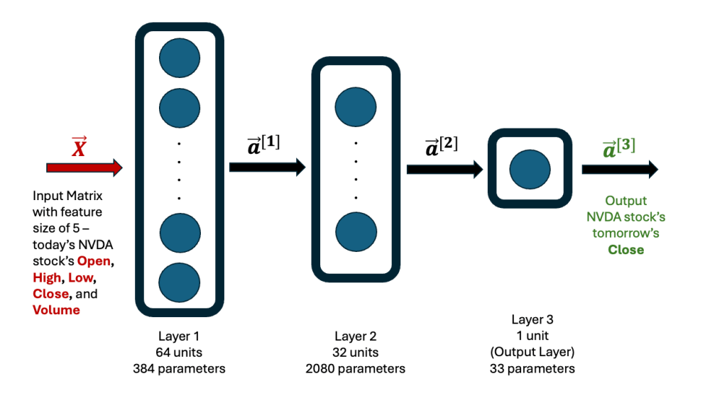
My neural network model takes in just 5 features per data point — the stock’s end-of-day Open, High, Low, Close, and Volume — to predict tomorrow’s Close price.

For training, I used NVDA’s stock data from January 1, 2020, to December 31, 2024 — a five-year period that includes 1,258 trading days. The target variable is the known next day’s Close price. The core idea was simple: Given today’s stock metrics for NVDA, can we predict tomorrow’s Close price?

The basic architecture of the neural network is a schema I’ve used many times before, and I’ve shared it here for clarity.

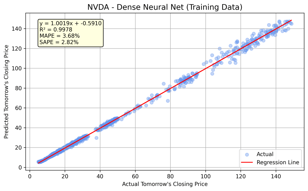
After training, the model learns all its weights and biases, totaling 2,497 parameters. It’s always a good idea to validate predictions made by a newly developed model — by running it on the training data and comparing the results with actual historical data. The graph below illustrates this comparison. The linear regression fit between the actual and predicted Close prices is excellent (R² = 0.9978). MAPE refers to the Mean Absolute Percentage Error, while SAPE is the Standard Deviation of the Percentage Error.

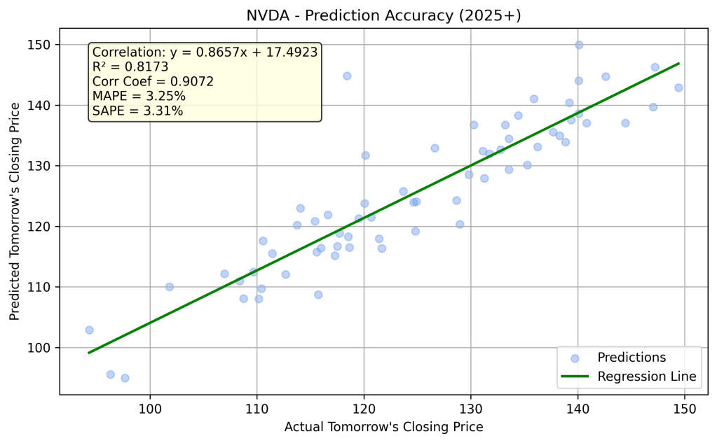
The trained model is now ready to predict NVDA’s closing price for the next trading day, based on today’s end-of-day data. I ran the model for every trading day in 2025, up to the date of writing this article: April 9, 2025 (using the known Close from April 8, 2025). The linear relationship between the actual and predicted Close prices for this period is shown in the following chart.

The correlation is reasonably strong (R² = 0.8173), though not as high as the model’s performance on the training set. On some days, the predictions are very accurate; on others, there are significant deviations. You’ll appreciate this better by examining the results in numerical and tabular form. The table below is a screenshot from the live implementation of the model, which you can run and explore on the Hugging Face Spaces platform. Update – please see a refined implementation at MLPowersAI, where you can see next day predictions for 5 stocks (AAPL, GOOGL, MSFT, NVDA, and TSLA).

The wild swings in closing prices — as reflected by large percentage errors — are mostly driven by market sentiment, which the model does not account for. For example, on April 3 and 4, 2025, the prediction errors were influenced by unexpected trade tariffs announced by the U.S. Government, which triggered strong market reactions.

Even though the percentage error swings wildly in 2025, we can still derive valuable insights from this lightweight neural network model by considering the MAPE bounds. For example, on March 28, 2025, the actual Close was $109.67, while the predicted Close was $113.11, resulting in a -3.14% error. However, based on all 2025 predictions to date, we know that the Mean Absolute Percentage Error (MAPE) is 3.25%. Using this as a guide for lower and upper bounds, the predicted Close range spans from $109.47 to $116.76.

We observe that the actual Close falls within these bounds. I strongly recommend reviewing the current table from the live implementation to make your own observations and draw conclusions.

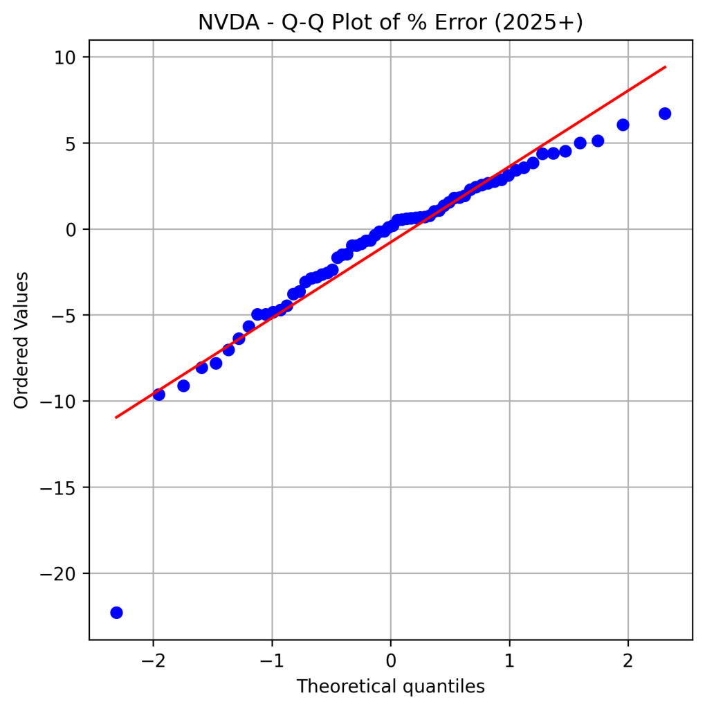
I was also curious to examine the distribution of the percentage error — specifically, whether it follows a normal distribution. The Shapiro-Wilk test (p-value = 0.0000) suggests that the distribution is not normal, while the Kolmogorov-Smirnov (K-S) test (p-value = 0.2716) suggests that it may be approximately normal. The data also exhibits left skewness and is leptokurtic. The histogram and Q-Q plot of the percentage error are shared below.

Another way to visualize the variation between the actual and predicted Close prices in 2025 is by examining the time series price plot, shown below.

Closing Thoughts …

Technical traders rely heavily on chart-based tools to guide their trades — support and resistance levels, moving averages, exponential trends, momentum indicators like RSI and MACD, and hundreds of other technical metrics. While these tools help in identifying trading opportunities at specific points in time, they don’t predict where a stock will close at the end of the trading day. In that sense, their estimates may be no better than the guess of a novice trader.

The average U.S. investor isn’t necessarily a technical day trader or an institutional analyst. And no matter how experienced a trader is, everyone is blind to the net market sentiment of the day. As the saying goes, the market discounts everything — it reacts to macroeconomic shifts, news cycles, political developments, and human emotion. Capturing all that in a forecast is close to impossible.

That’s where neural network-based machine learning models step in. By training on historical data, these models take a more mathematical and algorithmic approach — offering a glimpse into what might lie ahead. While not perfect, they represent a step in the right direction. My own lightweight model, though simple, performs remarkably well on most days. When it doesn’t, it signals that the model likely needs more input features.

To improve predictive power, we can expand the feature set beyond the five core inputs (Open, High, Low, Close, Volume). Additions like percentage return, moving averages (SMA/EMA), rolling volume, RSI, MACD, and others can enhance the model’s ability to interpret market behavior more effectively.

What excites me most is the democratization of this technology. Models like this one can help level the playing field between everyday investors and institutional giants. I foresee a future where companies emerge to build accessible, intelligent trading tools for the average person — tools that were once reserved for Wall Street.

I invite you to explore and follow the live implementation of this model. Observe how its predictions play out in real time. My personal belief is that neural networks hold immense potential in stock prediction — and we’re only just getting started.

Update (May 2025):
Since publishing this article, I have deployed a more advanced neural network model that forecasts next-day closing prices for five major stocks (AAPL, GOOGL, MSFT, NVDA, TSLA). The model runs daily and is hosted on a custom FastAPI and NGINX platform at MLPowersAI Stock Prediction.

Disclaimer

The information provided in this article and through the linked prediction model is for educational and informational purposes only. It does not constitute financial, investment, or trading advice, and should not be relied upon as such.

Any decisions made based on the model’s output are solely at the user’s own risk. I make no guarantees regarding the accuracy, completeness, or reliability of the predictions. I am not responsible for any financial losses or gains resulting from the use of this model.

Always consult with a licensed financial advisor before making any investment decisions.

Bringing Historical Process Data to Life: Unlocking AI’s Goldmine with Neural Networks for Smarter Manufacturing

In every factory, industrial operation, and chemical plant, vast amounts of process data are continuously recorded. Yet most of it remains unused, buried in digital archives. What if we could bring this hidden goldmine to life and transform it into a powerful tool for process optimization, cost reduction, and predictive decision-making? AI and machine learning (ML) are revolutionizing industries by turning raw data into actionable insights. From predicting product quality in real-time to optimizing chemical reactions, AI-driven process modeling is not just the future. It is ready to be implemented today.

In this article, I will explore how historical process data can be extracted, neural networks can be trained, and AI models can be deployed to provide instant and accurate predictions. These technologies will help industries operate smarter, faster, and more efficiently than ever before.

How many years of industrial process data are sitting idle on your company’s servers? It’s time to unleash it—because, with AI, it’s a goldmine.

I personally know of billion-dollar companies that have decades of process data collecting dust. Manufacturing firms have been diligently logging process data through automated DCS (Distributed Control Systems) and PLC (Programmable Logic Controller) systems at millisecond intervals—or even smaller—since the 1980s. With advancements in chip technology, data collection has only become more efficient and cost-effective. Leading automation companies such as Siemens (Simatic PCS 7), Yokogawa (Centum VP), ABB (800xA), Honeywell (Experion), Rockwell Automation (PlantPAx), Schneider Electric (Foxboro), and Emerson (Delta V) have been at the forefront of industrial data and process automation. As a result, massive repositories of historical process data exist within organizations—untapped and underutilized.

Every manufacturing process involves inputs (raw materials and energy) and outputs (products). During processing, variables such as temperature, pressure, motor speeds, energy consumption, byproducts, and chemical properties are continuously logged. Final product metrics—such as yield and purity—are checked for quality control, generating additional data. Depending on the complexity of the process, these parameters can range from just a handful to hundreds or even thousands.

A simple analogy: consider the manufacturing of canned soup. Process variables might include ingredient weights, chunk size distribution, flavoring amounts, cooking temperature and pressure profiles, stirring speed, moisture loss, and can-filling rates. The outputs could be both numerical (batch weight, yield, calories per serving) and categorical (taste quality, consistency ratings). This pattern repeats across industries—whether in chemical plants, refineries, semiconductor manufacturing, pharmaceuticals, food processing, polymers, cosmetics, power generation, or electronics—every operation has a wealth of process data waiting to be explored.

For companies, revenue is driven by product sales. Those that consistently produce high-quality products thrive in the marketplace. Profitability improves when sales increase and when cost of goods sold (COGS) and operational inefficiencies are reduced. Process data can be leveraged to minimize product rejects, optimize yield, and enhance quality—directly impacting the bottom line.

How can AI help?

The answer is simple: AI can process vast amounts of historical data and predict product quality and performance based on input parameters—instantly and with remarkable accuracy.

A Real-Life Manufacturing Scenario

Imagine you’re the VP of Manufacturing at a pharmaceutical company that produces a critical cancer drug—a major revenue driver. You’ve been producing this drug for seven years, ensuring a steady supply to patients worldwide.

Today, a new batch has just finished production. It will take a week for quality testing before final approval. However, a power disruption occurred during the run, requiring process adjustments and minor parts replacements. The process was completed as planned, and all critical data was logged. Now, you wait. If the batch fails quality control a week later, it must be discarded, setting you back another 40 days due to production and scheduling delays.

Wouldn’t it be invaluable if you could predict, on the same day, whether the batch would pass or fail? AI can make this possible. By training machine learning models on historical process data and batch outcomes, we can build predictive systems that offer near-instantaneous quality assessments—saving time, money, and resources.

Case Study: CSTR Surrogate AI/ML Model

To illustrate this concept, let’s consider a Continuous Stirred Tank Reactor (CSTR).

The system consists of a feed stream (A) entering a reactor, where it undergoes an irreversible chemical transformation to product (B), and both the unreacted feed (A) and product (B) exit the reactor.

$A \rightarrow B$

The process inputs are the feed flow rate F (L/min), concentration CA_in (mol/L), and temperature T_in (K, Kelvin).

The process outputs of interest are the exit stream temperature, T_ss (K) and the concentration of unreacted (A), CA_ss (K). Knowing CA_ss is equivalent to knowing the concentration of (B), since the two are related through a straight forward mass balance.

The residence time in the CSTR is designed such that the output has reached steady state conditions. The exit flow rate is the same as the input feed flow rate, since it is a continuous and not a batch reactor.

Generating Data for AI Training

To develop an AI/ML model we would need training data. We could do many experiments and gather the data, in lieu of historical data. However, this CSTR illustration was chosen, since we can generate the output parameters through simulation. Further, this problem has an analytical steady state solution, which can be used for further accuracy comparisons. The focus of this article is not to illustrate the mathematics behind this problem, and therefore, this delegated to a brief note at the end.

When historical data has not been collated from real industrial processes, or if it is unavailable, computer simulations can be run to estimate the output variables for specified input variables. There are more than 50 industrial strength process simulation packages in the market, and some of the popular ones are – Aspen Plus / Aspen HYSYS, CHEMCAD, gPROMS, DWSIM, COMSOL Multiphysics, ANSYS Fluent, ProSim, and Simulink (MATLAB).

Depending on the complexity of the process, the simulation software can take anywhere from minutes, to hours, or even days to generate a single simulation output. When time is a constraint, AI/ML models can serve as a powerful surrogate. Their prediction speeds are orders of magnitude faster than traditional simulation. The only caveat is that the quality of the training data must be good enough to represent the real world historical data closely.

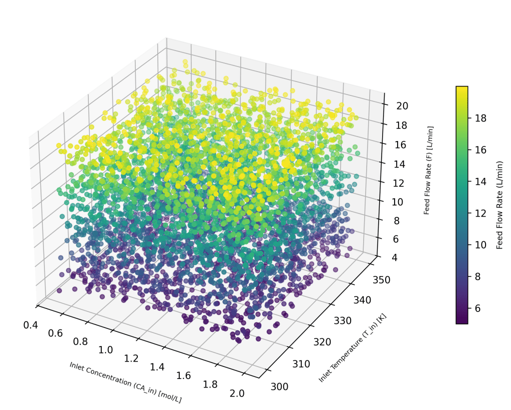
As explained in the brief note in the CSTR Mathematical Model section below, this illustration has the advantage of generating very reliable outputs, for any given set of input conditions. For developing the training set, the input variables were varied in the following ranges.

CA_in = 0.5 – 2.0 mol/L

T_in = 300 – 350 K (27 – 77 C)

F = 5 – 20 L/min

Each of the training sets have these 3 input variables. 5000 random feature sets (X) were generated using a uniform distribution, and the 3D plot shows the variations.

For training the AI/ML model 80% of these feature sets were selected at random and used, while for testing 20% were used as the test set. The corresponding output variables, Y, (CA_ss, T_ss) were numerically calculated for each off the 5000 input feature sets, and were used for the respective training and testing.

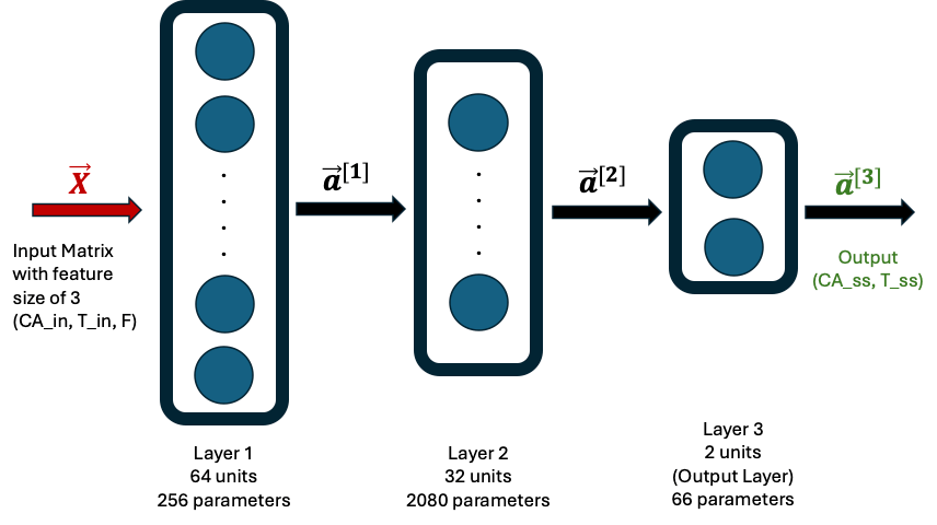
ML Neural Network Model

The ML model consisted of a Neural Network (NN) with 2 hidden layers and one output layer as follows. The first hidden layer had 64 neurons and the second one had 32 neurons. The final output layer had 2 neurons. The ReLU activation was used for the hidden layers and a linear activation for the output layer. The loss function used was mean-squared-error.

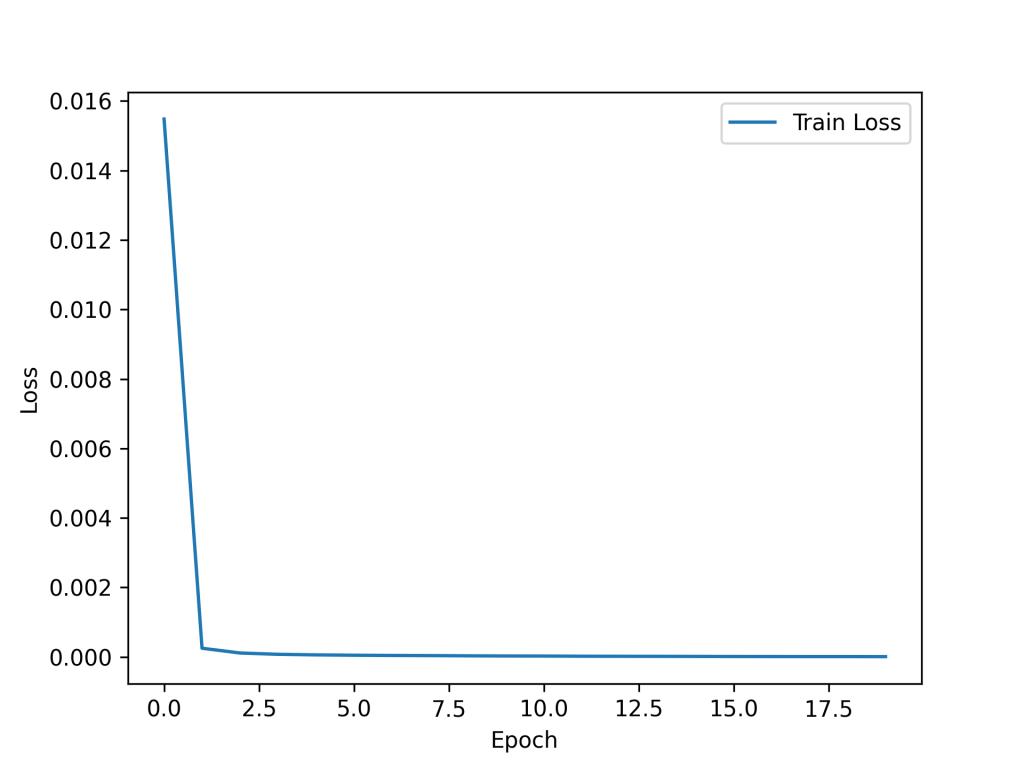
The model was trained on the training set for 20 epochs and showed rapid convergence. The loss vs epochs is presented here. The final loss was near zero (~10^-6).

After training the NN model, the Test Set was run. It yielded a Test Loss of zero (rounded off to 4 decimal places) and a Test MAE (mean average error) of 0.0025. The model has performed very nicely on the Test Set.

AI/ML Model Inference

This is where AI/ML gets really exciting! I’ve packaged and deployed the neural network model on Hugging Face Spaces, using Gradio to create an interactive and web-accessible interface. Now, you can take it for a test drive—just plug in the input values, hit Submit, and watch the predictions roll in!

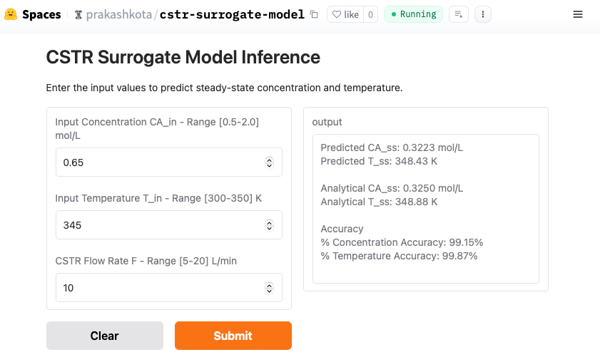
An actual output (screen shot) from a sample inference is shown here for input values which are within the range of the training and test sets. Both outputs (CA_ss and T_ss) are over 99% accurate.

However, this might not be all that surprising, considering the training set—comprising 4,000 feature sets (80% of 5,000)—covered a wide range of possibilities. Our result could simply be close to one of those existing data points. But what happens when we push the boundaries? My response to that would be to test a feature set where some values fall outside the training range.

For instance, in our dataset, the temperature varied between 300–350 K. What if we increase it by 10% beyond the upper limit, setting it at 385 K? Plugging this into the model, we still get an inference with over 99% accuracy! The predicted steady-state temperature (T_ss) is 385.35 K, compared to the analytical solution of 388.88 K, yielding an accuracy of 99.09%. A screenshot of the results is shared below.

Summary

I’m convinced that AI/ML has remarkable power to predict real-world scenarios with unmatched speed and accuracy. I hope this article has convinced you too. Within every company lies a hidden treasure trove of historical process data—an untapped goldmine waiting to be leveraged. When this data is extracted, cleaned, and harnessed to train a custom ML model, it transforms from an archive of past events into a powerful tool for the future.

The potential benefits are immense: vastly improved process efficiency, enhanced product quality, smarter process optimization, reduced downtime, better scheduling and planning, elimination of guesswork, and increased profitability. Incorporating ML into industrial processes requires effort—models must be carefully designed, trained, and deployed for real-time inference. While there may be cases where a single ML model can serve multiple organizations, we are still in the early stages of AI/ML adoption in process industries, and these scalable use cases are yet to be fully explored.

Right now, the opportunity is massive. The companies that act today—dusting off their historical data, building custom AI models, and integrating ML into their operations—will set the standard and lead their industries into the future. The question is: Will your company be among them?

CSTR Mathematical Model

Read this section only if you like math and want the details!

The mass and energy balance on the CSTR yield the following equations, which give the variation of concentration for the reacting species (A) and the fluid temperature (T) as a function of time (t).

$\frac{dC_A}{dt} = \frac{F}{V} (C_{A,\text{in}} - C_A) - k C_A$

$\frac{dT}{dt} = \frac{F}{V} (T_{\text{in}} - T) + \frac{-\Delta H}{\rho C_p} k C_A$

$C_A$ and $T$ are the exit concentration of A and fluid temperature $T$ . Since the residence time is long enough to reach steady state, for this irreversible reaction,

$C_A =$ CA_ss

$T =$ T_ss

The following model parameters have been taken to be a constant for all the simulated runs and analytical calculations. There is no requirement to have physical properties to be constant, since they could be allowed to vary with temperature. However, for this simulation they have been held constant.

$V =$ 100 L (tank volume)

${\Delta H} =$ -50,000 J/mol (heat of exothermic reaction)

${\rho} =$ 1 Kg/L (fluid density)

$C_p =$ 4184 J/Kg.K (fluid specific heat capacity)

The irreversible reaction for species (A) going to (B) is modeled as a first order rate equation, with the rate constant $k =$ 0.1 min^-1, and where $-r_A$ is the reaction rate (mol/L.min).

$-r_A = kC_A$

I have used a mix of SI and common units. However, when taken together in the equation, the combined units work consistently.

The analytical solution is easy to calculate and can be done by setting the time derivatives to zero and solving for the concentration and temperature. These are provided here for completeness.

CA_ss $= \frac{F C_{A,\text{in}} }{F + k V}$

T_ss = T_in – $\frac{\Delta H k C_A V}{\rho C_p F}$

To simulate the training set, we can calculate CA_ss and T_ss from the above equations. I have computed CA_ss and T_ss by solving the system of ordinary differential equations using scipy.integrate.solve_ivp, which is an adaptive-step solver in SciPy. The steady state values were taken as the dependent variable values after a lapse time of 50 minutes. These values would vary slightly from analytical values. But, they provide small variations, just like in real processes due to inherent fluctuations.

The Power of Machine Learning in Medical Diagnosis – Breast Cancer Mini Case using Neural Networks

Medical misdiagnoses continue to be a significant concern worldwide, often leading to unnecessary complications and preventable deaths. According to the World Health Organization (WHO), at least 5% of adults in the U.S. experience a diagnostic error annually. The impact on a global scale is even more alarming. Despite rapid advancements in Artificial Intelligence (AI) and Machine Learning (ML), adoption in clinical settings remains limited. Many healthcare professionals remain skeptical, with only 3% of European healthcare organizations expressing trust in AI-enabled diagnostics. This blog explores the application of Neural Networks in breast cancer detection using the Wisconsin Breast Cancer Dataset. It examines how TensorFlow based models can improve diagnostic accuracy and assesses the potential of AI-driven systems in medical practice

Have you felt rushed in a doctor’s office? Have you ever left an appointment wondering if the doctor thoroughly reviewed your blood test results and other relevant information? Have you doubted the Doctor’s opinion? You are not alone!

In a 2019 World Health Organization (WHO) article, WHO states that their research shows that at least 5% of adults in the United States experience a diagnostic error each year in outpatient settings. In a 2023 article in BMJ, the authors state that there are 2.59 million missed diagnoses in the US, accounting for 371,000 deaths and 424,000 disabilities. These numbers are for only the false negative errors. When considered on a global scale, the numbers are staggering.

Whatever may be the reason for the errors in medical diagnosis, it’s obvious that these numbers must come down. Most doctors that I have met for a professional consultation, for myself or my family members, have advised me not to ‘Google’ medical conditions. At the same time, they do not have enough of time or patience to explain the condition. I can’t blame them, considering their patient load and time constraints.

The enormous interest in AI and Machine Learning, in all walks of life, is a tool that doctors should be using daily to minimize errors in medical diagnosis. I had assumed that this is happening at a rapid pace. But I was so wrong on this. In a 2022 article in the Frontiers in Medicine, the authors conclude that from their survey of medical professionals in 39 countries, 38% had awareness of clinical AI, but that 53% lacked basic knowledge of clinical AI. Their work also revealed that 68% of doctors disagreed that AI would become a surrogate physician, but they believed that AI should assist in clinical decision making. In a 2024 online summary, it is mentioned that 42% of healthcare organizations in the European Union were currently using AI technologies for disease diagnosis, but that only 3% trusted AI-enabled decisions in disease diagnostics. These pieces of information only indicate that the adoption of AI for disease diagnosis is under suspicion by the professionals. If anything, the adoption is slow, though the advancement in AI and Machine Learning has been very rapid. There is a trust and acceptance deficit when it comes to AI/ML in medical practice. Integration of AI/ML into clinical workflows would be the next big challenge. Finally, regulatory approvals would be a barrier to AI/ML implementation in medical establishments. But these hurdles will be overcome in due time, hopefully sooner rather than later.

I like to work on small cases when confronted with big questions such as this one. I’ll share with you a case that is based on Breast Cancer. American Cancer Society estimates that Approximately 1 in 8 women in the US (13.1%) will be diagnosed with invasive breast cancer, and 1 in 43 (2.3%) will die from the disease. Breastcancer.org estimates that approximately 310,720 women are expected to be diagnosed with invasive breast cancer annually in the US. Stopbreastcancer.org estimates that the mortality rate in the US is about 42,170 annually. WHO reports that in 2022 approximately 2.3 million women worldwide were diagnosed with breast cancer, accounting for 11.6% of all cancer cases globally. Further, it reported 670,000 breast cancer related deaths in 2022.

Doctors use a variety of techniques to detect breast cancer – mammography, breast ultrasound, PET scans, DNA sequencing and biopsies. A biopsy, which is a small extraction of a physical sample for microscope analysis, is a standard investigation tool. The investigations are performed by pathologists. The output from this analysis are measurements and metrics that capture features, giving the pathologists a means to reliably diagnose whether the lesions are malignant or benign.

A reputed biopsy database, based on the fine needle aspiration technique, is the Diagnostic Wisconsin Breast Cancer Database. It contains data for 569 patient biopsies, with each data set having 30 measurement features, shown here.

id, diagnosis, radius_mean, texture_mean, perimeter_mean, area_mean, smoothness_mean, compactness_mean, concavity_mean, concave_points_mean, symmetry_mean, fractal_dimension_mean, radius_se, texture_se, perimeter_se, area_se, smoothness_se, compactness_se, concavity_se, concave_points_se, symmetry_se, fractal_dimension_se, radius_worst, texture_worst, perimeter_worst, area_worst, smoothness_worst, compactness_worst, concavity_worst, concave_points_worst, symmetry_worst, fractal_dimension_worst

The header contains 32 categories, but the first column is the patient ID and the second column is the actual diagnosis, M is for malignant and B is for benign. Excluding this header and the first 2 columns, the data is a matrix of size (569,30). With 30 pieces of input data for a single biopsy for a patient, it seems daunting for a pathologist to look at all of them, in its entirety, to diagnose whether a biopsy is cancerous or not. For example, the large input feature set for the first patient, based on actual data in the data set, is shown here to give you an idea of the volume of data to consider before a diagnosis.

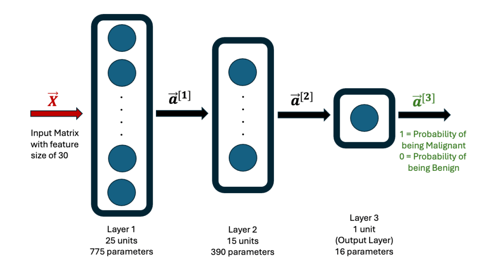
842302,M,17.99,10.38,122.8,1001,0.1184,0.2776,0.3001,0.1471,0.2419,0.07871,1.095,0.9053,8.589,153.4,0.006399,0.04904,0.05373,0.01587,0.03003,0.006193,25.38,17.33,184.6,2019,0.1622,0.6656,0.7119,0.2654,0.4601,0.1189

Using this dataset, a Neural Network algorithm for Structured Machine Learning was created, using TensorFlow. The Jupyter Notebook Python code is on Github. The Neural Network consists of 3 hidden layers, the first one with 25 neurons (units), the second one with 15 neurons and the third one with 1 neuron. The first two layers use the ReLU function, while the last one uses the Sigmoid function. The architecture is shown here.

Rows 26 to 569 in the breast cancer data set were used as the Training set, while the first 25 rows were used as the Test set. The former is used to establish the weights and biases in each neuron in the network. The final output is either a 1 or 0, with 1 indicating that the data corresponds to a malignant diagnosis, while a 0 corresponds to a benign diagnosis.

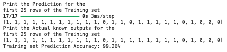
After running the Neural Network code, the model was used to predict outputs for the entire Training set. Since the Training set contains the actual diagnosis (1 = M = Malignant) and (0 = B = Benign), it can be compared to the predicted output, to compute the accuracy of the Neural Network model. The model predicts a 99.26% accuracy. The predicted versus the actual output for the first 25 rows of the Training set is shown here. For the 15th row, the model predicts the outcome as 0, while the actual outcome is 1. Hence, the overall accuracy over the entire Training set is less than 100%, but still remarkable at 99.26%.

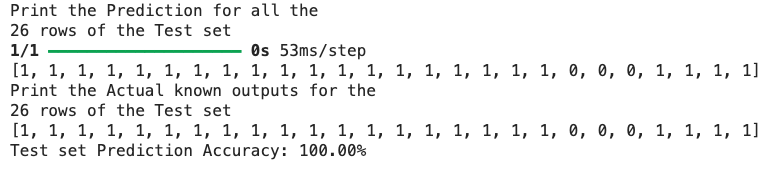
Next, the same model is used to predict the outcome for the Test set. The model has never seen this Test set before. It is equivalent to new patient data coming from the field. The prediction from the model for the Test set shows an accuracy of 100%! For comparison, the entire 26 rows of the predicted versus actual outcomes for the Test set is shown here.

These results are stunning. It emphatically shows the power of Machine Learning algorithms. For this specific case study, with a Training set of 543 patient records, it is possible to predict the cancer diagnosis for any new patient record, with an extremely high degree of accuracy.

With the number of tests that doctors ask patients to go through, hundreds of data values are generated. To make sense of all these data values, data analytics is required, rather than reliance on a cursory glance by a doctor. Neural Networks and Supervised Machine Learning are powerful AI tools that will benefit the patient today. AI can be applied to any disease diagnosis, for which raw data exists. Its adoption for reliable medical diagnosis is the need of the hour.

For those interested, the breast cancer dataset can also be analyzed using a Logistics Regression algorithm, using the Scikit-learn package. This code has also been provided on Github. The results are comparable to the Neural Network algorithm. Another small note – the TensorFlow package is one among several options available for writing Neural Networks code. Other choices are PyTorch (Meta), JAX (Google), MXNet (Apache) and CNTK (Microsoft).

You can take the Model for a test spin on the Hugging Face Platform – Breast Cancer Neural Network Prediction

Can you use ChatGPT, Gemini or Copilot to train Linear Regression Models with Gradient Descent?

Linear regression, one of the simplest and most foundational tools in machine learning, is widely used to predict outcomes based on input features. While custom coding has traditionally been the go-to method for solving linear regression problems, the emergence of Large Language Models (LLMs) like OpenAI’s ChatGPT, Google’s Gemini, and Microsoft’s Copilot has opened up exciting new possibilities. Can these LLMs generate accurate and usable code for linear regression models? This post explores that question in detail, using a dataset to predict house prices based on features such as size, number of bedrooms, number of floors and age. Python code generated by these LLMs and their outputs are compared, and their ability to scale and handle real-world constraints is examined.

LLMs and Linear Regression: A Deep Dive

One can always write a custom code to fit training sets to a Linear Regression Model. But, instead, can’t we just use publicly available LLMs (Large Language Models) such as OpenAI’s ChatGPT, Google Gemini or Microsoft Copilot?

All three LLMs were tasked with generating Python code using the Scikit-learn package and the gradient descent method using the following prompt.

Attached is a csv file called houses.99.txt and it is delimited by “,”. The first row is a header. The remainder rows contain the numerical data. The first four columns contain the input features, X_train, which are for predicting the house prices. The fifth column contains the house prices in units of 1000’s of dollars, y_train. We wish to fit a linear model y = w.X + b, where w are the weights, b is the bias value and X is the input feature set and y is the output house price in dollars. Please give a python code to determine the linear model for X_train and y_train using sklearn and the SGDRegressor. Use scaling for X_train. Please also include the code for reading X_train and y_train from the houses99.txt file. Using this code, determine the weights and bias and show the model. Calculate the weights and the bias using this code, and give the model. Print the mean and standard deviation, for each column in X_train. Finally, predict the house price for a new feature set [1200, 3, 1, 40]. Give the scaled values for this feature set. Also, provide the python code listing and let the print statements for numbers be to 8 decimal places.

A short synopsis on the Linear Regression Model is provided at the bottom for quick review. The Python code and supporting files used in this blog evaluation are available on GitHub.

Dataset Details

The houses99.txt file is a training set file that has 99 training sets. Each training set has 4 features x1 (sft), x2 (number of bedrooms), x3 (number of floors) and x4 (age in years); and 1 output for house price y ($ in 1000’s). For example:

	x1 (sft)	x2 (rooms)	x3 (floors)	x4 (age)	y ($ in 1000’s)
1st set	1244	3	1	64	300
2nd set	1947	3	2	17	510

Code Generation and Results

The objective of the prompt is to generate a linear model of the type shown here and the equation is described in the short synopsis later on in this post.

$\hat{y} = w1*x1 + w2*x2+ w3*x3 + w4*x4 + b$

All three LLMs (ChatGPT, Gemini, and Copilot) successfully generated Python code. After running the code locally, the outputs were compared. Here are the weights and bias values they produced:

	w1	w2	w3	w4	b
ChatGPT	110.280	-21.130	-32.545	-38.012	363.163
Gemini	110.280	-21.130	-32.545	-38.012	363.163
Copilot	110.312	-21.142	-32.574	-38.000	363.163

Taking the ChatGPT model as an example, the fitted model is:

$\hat{y} = 110.280*x1 -21.130*x2 - 32.545*x3 - 38.012*x4 + 363.163$

Predictions

The above model can be used to now predict the house price. For example, for a test feature set X = [1200, 3, 1, 40], the model predicts a price of $318,793.95.

It is important to note that directly substituting the raw feature values into the model will not yield the predicted result shown. This discrepancy arises because the code applies standard normalization using the StandardScaler from sklearn.preprocessing. In this process, each data value in a column is scaled relative to the column’s mean and standard deviation. Following normalization, the column is transformed to have a mean of 0 and a standard deviation of 1. This scaling step is a necessary mathematical requirement for linear regression to ensure consistent and accurate model performance.

The before and after scaling values for the feature set X = [1200, 3, 1, 40] is shown here.

X =	x1 (sft)	x2 (rooms)	x3 (floors)	x4 (age)
Unscaled	1200	3	1	40
Scaled	-0.53052829	0.43380884	-0.78927234	0.06269567

If the scaled values of X are substituted in the model, the predicted value is $318,793.95. This seems like a lit bit of extra work and knowledge, and we know that the code can do all this scaling behind the scenes. But, would it not be nice to ask the LLMs to do this as well?

LLMs ability to run code

As of now, Microsoft Copilot has no mechanism from within its chat interface to upload the training data set (houses99.txt). But, if the python code has to be run, it can be done on Microsoft’s Azure cloud platform. There is no simple way to run.

ChatGPT provides the ability to upload the training data set. After uploading, and asking it run the model prompt, it can be tasked to predict the house prices for the test training set, [1200, 3, 1, 40]. ChatGPT would do the necessary conversions and give the result, like the one shown here. This is quite cool!

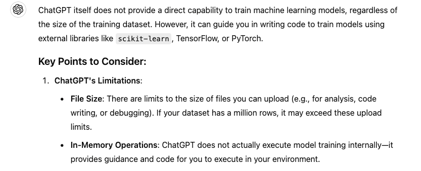
It would be difficult to do this on the free tier of ChatGPT. By subscribing to the Plus tier, which costs about $20/month, file upload is enabled. However, it is also not possible to upload a very large training set, say with a thousand or million training data sets. This is what ChatGPT had to say on this matter.

For very large training data sets, it would be practical to run the code on a custom environment, where one had total control of the computing power, memory and data management. But, for small data sets, at least for the sizes used in this experiment, we can accomplish some quick analysis on this LLM.

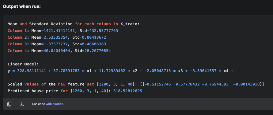
Google’s Gemini does not have a mechanism to upload a file for analysis. However, Gemini Advanced offers such services, but it is subscription based ($19.99/month). Google is also offering a code writing and testing platform called Google AI Studio, which is free at the moment. But, I’m sure it will be subscription based soon. I was able to run the prompt on the Google AI Studio and also run it. Here are the results.

The code upon running has given a linear model with w and b values that are very different from that obtained when the same code is run on a local computer, as shown in the earlier table. However, it predicts the correct price of $318,528.12 for the new feature set [1200, 3, 1, 40]. Its in the same ballpark as the code run on an independent computer. However, since the weights and bias values are similar when the code from each of the three LLMs are run on the same computer, I would personally not rely on the code output given by Google AI Studio.

Summary

All three public LLMs – ChatGPT, Gemini and Copilot generate excellent python code to predict a linear regression model by the gradient descent method and the Scikit-learn package. When the codes are run on the same computer, they produce weights and bias values that are identical. They also predict the output correctly for a new input feature set. ChatGPT and Google AI Studio can run the python code from within the chat window, for small data sets, such as the 99 training sets in our experiment. However, for larger training sets, we have to use custom computing environments. Microsoft pilot does not offer any free tier service to upload and test models. Nevertheless, the ability for all three LLMs to write code correctly is impressive.

Linear Regression Models – a quick review…

We try to predict things every day. The weather channel predicts the temperature. The financial analyst predicts the future value of the stock price. The airlines predict the time of arrival of an aircraft. We live in a world filled with predictions. How is it done?

One way is to make a random guess. But, this has a very low probability of being correct. We are not fortune tellers! Another way is to create a model to predict an output ‘y’ for a given set of input features ‘X’. We could write the relationship as:

$y = \text{function}(X) = f(X)$

In real world problems the feature set ‘X’ would be one or more input variables. For example, we may want to predict the house price (y) given its sft, number of bedrooms, number of floors and its age. Here, the feature set X has 4 input variables – x1, x2, x3 and x4. Mathematically this is called as a 1D array of 4 variables. We could write it as:

$\mathbf{X} = \{x1, x2, x3, x4\}$

But, what is the function that can predict y?

A well known function is a model based on Linear Regression and it is written as follows:

$\hat{y} = w1*x1 + w2*x2+ w3*x3 + w4*x4 + b$

In short form it is written as $\hat{y} = \mathbf{w} \cdot \mathbf{X} + b$ , where w is a 1-D vector and X is a matrix. Here, y has a funny upward pointing arrow symbol, called as y-hat, indicating that it is a predicted value. Further, w.X is known as the dot product of vector w with matrix X. In this illustration, the matrix X is a 1-D vector, since we are dealing with only one feature set. The math challenge is to determine w1, w2, w3 and w4, which are called as the model weights, and to determine, b, which is known as the bias. There are 5 unknowns and if we had 5 equations, the unknowns could be solved for simultaneously. For example, if we had the data for 5 houses, we could generate 5 equations based on the model. Therefore, we can develop a model prediction for y. However, it would be an equation that would satisfy the 5 feature sets, i.e. given one of the 5 known feature sets, it would give an estimate for $\hat{y}$ .

What if we had a data set for 10,000 houses? You can imagine this as a 10,000 row data set in MS Excel, with each data row having 5 columns, 4 for the X data and 1 for the y data. This is a 2-D array of size 10,000 rows x 5 columns, which is a matrix of size (10000×5). Would the linear model work and fit all the 10,000 data rows for some unique values of w (i.e. w1, w2, w3 and w4) and b? Of course, the earlier values of w determined with 5 feature sets is unlikely to work for the 10,000 data set, since the problem is overdetermined. Instead, in linear regression, a best fit is established by choosing w iteratively, so that the square of the error between the real value (y) and the predicted value $\hat{y}$ is minimized. This is called as the least square method.

If linear regression is applied to the 10,000 data set problem (each called a training set), the error is based on the least squares method, but it is summed over all the training sets. This summed value is known as the “Cost Function” in the language of Machine Language (ML). One popular technique to iteratively compute the weights w and the bias b, is known as the Gradient Descent (GD) method. This type of linear model, where the linear regression model is fit to a training data set is popularly known as Supervised Learning in ML and AI.

Acknowledgements

The houses99.txt data file has been adopted from the data set used in the course Supervised Machine Learning: Regression and Classification by Andrew Ng, which is offered jointly by Stanford University Online and DeepLearning.AI, through Coursera. This is an excellent course for learning Machine Learning through writing code and algorithms.